Progressively adding potassium feldspar
This page follows Chapter 13 of Bethke (2007) and involves computing the equilibrium system as K-feldspar is added to a hypothetical water.
The initial composition of the water is shown in Table 1. Assume that the temperature is 25C and the initial pH is 5. cm of K-feldspar is slowly added to this system.
Table 1: Initial bulk composition of the hypothetical water
| Species | Concentration (molal) | Approx conc (mg/kg(solvent water)) |
|---|---|---|
| HCO | 50 | |
| Cl | 30 | |
| Ca | 15 | |
| SO | 8 | |
| Na | 5 | |
| Mg | 3 | |
| SiO(aq) | 3 | |
| K | 1 | |
| Al |
MOOSE input file: definition
The GeochemicalModelDefinition specifies the database file to use, and in this case the basis species and equilibrium minerals. The flag piecewise_linear_interpolation = true in order to compare with the Geochemists Workbench result
[UserObjects<<<{"href": "../../../syntax/UserObjects/index.html"}>>>]
  [definition]
    type = GeochemicalModelDefinition<<<{"description": "User object that parses a geochemical database file, and only retains information relevant to the current geochemical model", "href": "../../../source/userobjects/GeochemicalModelDefinition.html"}>>>
    database_file<<<{"description": "The name of the geochemical database file"}>>> = "../../../database/moose_geochemdb.json"
    basis_species<<<{"description": "A list of basis components relevant to the aqueous-equilibrium problem. H2O must appear first in this list.  These components must be chosen from the 'basis species' in the database, the sorbing sites (if any) and the decoupled redox states that are in disequilibrium (if any)."}>>> = "H2O H+ Na+ K+ Ca++ Mg++ Al+++ SiO2(aq) Cl- SO4-- HCO3-"
    equilibrium_minerals<<<{"description": "A list of minerals that are in equilibrium with the aqueous solution.  All members of this list must be in the 'minerals' section of the database file"}>>> = "K-feldspar Kaolinite Muscovite Quartz Phengite"
    piecewise_linear_interpolation<<<{"description": "If true then use a piecewise-linear interpolation of logK and Debye-Huckel parameters, regardless of the interpolation type specified in the database file.  This can be useful for comparing with results using other geochemistry software"}>>> = true # for comparison with GWB
  []
[]MOOSE input file: initial conditions and reaction rates
The TimeDependentReactionSolver defines the initial conditions and the desired reaction processes:
The pH is defined through specifying the
activityfor H. Note that at time zero, just after the initial equilibration, this activity constraint is removed via theremove_fixed_activityinputs.The bulk composition of the other chemical species are specified by the
moles_bulk_species, as per Table 1.The rate of addition of
K-feldsparis defined to be mol/s, which corresponds to cm/s.The other flags are for efficiency and enable an accurate comparison with the Geochemists Workbench software.
[TimeDependentReactionSolver<<<{"href": "../../../syntax/TimeDependentReactionSolver/index.html"}>>>]
  model_definition<<<{"description": "The name of the GeochemicalModelDefinition user object (you must create this UserObject yourself)"}>>> = definition
  geochemistry_reactor_name<<<{"description": "The name that will be given to the GeochemistryReactor UserObject built by this action"}>>> = reactor
  charge_balance_species<<<{"description": "Charge balance will be enforced on this basis species.  This means that its bulk mole number may be changed from the initial value you provide in order to ensure charge neutrality.  After the initial swaps have been performed, this must be in the basis, and it must be provided with a bulk_composition constraint_meaning."}>>> = "Cl-"
  constraint_species<<<{"description": "Names of the species that have their values fixed to constraint_value with meaning constraint_meaning.  All basis species (after swap_into_basis and swap_out_of_basis) must be provided with exactly one constraint.  These constraints are used to compute the configuration during the initial problem setup, and in time-dependent simulations they may be modified as time progresses."}>>> = "H2O              H+            Na+              K+               Ca++             Mg++             Al+++            SiO2(aq)         Cl-              SO4--            HCO3-"
  constraint_value<<<{"description": "Numerical value of the containts on constraint_species"}>>> = "  1.0              -5            5                1                15               3                1                3                30               8                50"
  constraint_meaning<<<{"description": "Meanings of the numerical values given in constraint_value.  kg_solvent_water: can only be applied to H2O and units must be kg.  bulk_composition: can be applied to all non-gas species, and represents the total amount of the basis species contained as free species as well as the amount found in secondary species but not in kinetic species, and units must be moles or mass (kg, g, etc).  bulk_composition_with_kinetic: can be applied to all non-gas species, and represents the total amount of the basis species contained as free species as well as the amount found in secondary species and in kinetic species, and units must be moles or mass (kg, g, etc).  free_concentration: can be applied to all basis species that are not gas and not H2O and not mineral, and represents the total amount of the basis species existing freely (not as secondary species) within the solution, and units must be molal or mass_per_kg_solvent.  free_mineral: can be applied to all mineral basis species, and represents the total amount of the mineral existing freely (precipitated) within the solution, and units must be moles, mass or cm3.  activity and log10activity: can be applied to basis species that are not gas and not mineral and not sorbing sites, and represents the activity of the basis species (recall pH = -log10activity), and units must be dimensionless.  fugacity and log10fugacity: can be applied to gases, and units must be dimensionless"}>>> = "kg_solvent_water log10activity bulk_composition bulk_composition bulk_composition bulk_composition bulk_composition bulk_composition bulk_composition bulk_composition bulk_composition"
  constraint_unit<<<{"description": "Units of the numerical values given in constraint_value.  Dimensionless: should only be used for activity or fugacity constraints.  Moles: mole number.  Molal: moles per kg solvent water.  kg: kilograms.  g: grams.  mg: milligrams.  ug: micrograms.  kg_per_kg_solvent: kilograms per kg solvent water.  g_per_kg_solvent: grams per kg solvent water.  mg_per_kg_solvent: milligrams per kg solvent water.  ug_per_kg_solvent: micrograms per kg solvent water.  cm3: cubic centimeters"}>>> = "   kg               dimensionless mg               mg               mg               mg               ug               mg               mg               mg               mg"
  source_species_names<<<{"description": "The name of the species that are added at rates given in source_species_rates.  There must be an equal number of these as source_species_rates."}>>> = "K-feldspar"
  source_species_rates<<<{"description": "Rates, in mols/time_unit, of addition of the species with names given in source_species_names.  A negative value corresponds to removing a species: be careful that you don't cause negative mass problems!"}>>> = "1.37779E-3" # 0.15cm^3 of K-feldspar (molar volume = 108.87 cm^3/mol) = 1.37779E-3 mol
  remove_fixed_activity_name<<<{"description": "The name of the species that should have their activity or fugacity constraint removed at time given in remove_fixed_activity_time.  There should be an equal number of these names as times given in remove_fixed_activity_time.  Each of these must be in the basis and have an activity or fugacity constraint"}>>> = "H+"
  remove_fixed_activity_time<<<{"description": "The times at which the species in remove_fixed_activity_name should have their activity or fugacity constraint removed."}>>> = 0
  ramp_max_ionic_strength_initial<<<{"description": "The number of iterations over which to progressively increase the maximum ionic strength (from zero to max_ionic_strength) during the initial equilibration.  Increasing this can help in convergence of the Newton process, at the cost of spending more time finding the aqueous configuration."}>>> = 0 # not needed for this simple problem
  stoichiometric_ionic_str_using_Cl_only<<<{"description": "If set to true, the stoichiometric ionic strength will be set equal to Cl- molality (or max_ionic_strength if the Cl- molality is too big).  This flag overrides ionic_str_using_basis_molality_only"}>>> = true # for comparison with GWB
  execute_console_output_on<<<{"description": "When to execute the geochemistry console output"}>>> = '' # only CSV output for this example
[]MOOSE input file: time stepping
A total of 100 steps over the course of 1s is used in this simulation
[Executioner<<<{"href": "../../../syntax/Executioner/index.html"}>>>]
  type = Transient
  dt = 0.01
  end_time = 1
[]MOOSE input file: outputs
A set of Postprocessors captures the output, using the AuxVariables added automatically by the TimeDependentReactionSolver:
[Postprocessors<<<{"href": "../../../syntax/Postprocessors/index.html"}>>>]
  [cm3_K-feldspar]
    type = PointValue<<<{"description": "Compute the value of a variable at a specified location", "href": "../../../source/postprocessors/PointValue.html"}>>>
    point<<<{"description": "The physical point where the solution will be evaluated."}>>> = '0 0 0'
    variable<<<{"description": "The name of the variable that this postprocessor operates on."}>>> = 'free_cm3_K-feldspar'
  []
  [cm3_Kaolinite]
    type = PointValue<<<{"description": "Compute the value of a variable at a specified location", "href": "../../../source/postprocessors/PointValue.html"}>>>
    point<<<{"description": "The physical point where the solution will be evaluated."}>>> = '0 0 0'
    variable<<<{"description": "The name of the variable that this postprocessor operates on."}>>> = 'free_cm3_Kaolinite'
  []
  [cm3_Muscovite]
    type = PointValue<<<{"description": "Compute the value of a variable at a specified location", "href": "../../../source/postprocessors/PointValue.html"}>>>
    point<<<{"description": "The physical point where the solution will be evaluated."}>>> = '0 0 0'
    variable<<<{"description": "The name of the variable that this postprocessor operates on."}>>> = 'free_cm3_Muscovite'
  []
  [cm3_Quartz]
    type = PointValue<<<{"description": "Compute the value of a variable at a specified location", "href": "../../../source/postprocessors/PointValue.html"}>>>
    point<<<{"description": "The physical point where the solution will be evaluated."}>>> = '0 0 0'
    variable<<<{"description": "The name of the variable that this postprocessor operates on."}>>> = 'free_cm3_Quartz'
  []
  [cm3_Phengite]
    type = PointValue<<<{"description": "Compute the value of a variable at a specified location", "href": "../../../source/postprocessors/PointValue.html"}>>>
    point<<<{"description": "The physical point where the solution will be evaluated."}>>> = '0 0 0'
    variable<<<{"description": "The name of the variable that this postprocessor operates on."}>>> = 'free_cm3_Phengite'
  []
[]Results
Bethke (2007) predicts that the minerals kaolinite, muscovite, quartz, K-feldspar and phengite all precipitate, and that kaolinite dissolves, as the K-feldspar is gradually added to the solution and the results are presented in Bethke (2007) Figure 13.1. These results are faithfully reproduced by the geochemistry module, as in Figure 1.
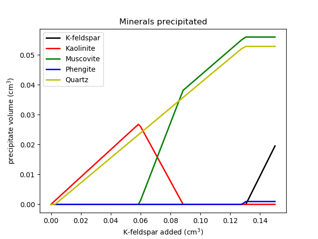
Figure 1: Minerals precipitated as K-feldspar is added to the system.
References
- Craig M. Bethke.
Geochemical and Biogeochemical Reaction Modeling.
Cambridge University Press, 2 edition, 2007.
doi:10.1017/CBO9780511619670.[Export]