Flow Over a Pebble
In this tutorial, you will learn how to:
Generate a mesh for NekRS
Create NekRS input files for laminar flow in dimensional form
Visualize NekRS outputs
To access this tutorial,
cd cardinal/tutorials/pebble_1
Geometry and Computational Model
The domain consists of a single pebble of diameter cm within a rectangular box; the pebble origin is at . Figure 1 shows the fluid portion of the domain (the pebble is not shown). The sideset numbering in the fluid domain is:
2: inlet
3: outlet
4: pebble surface
5: side walls
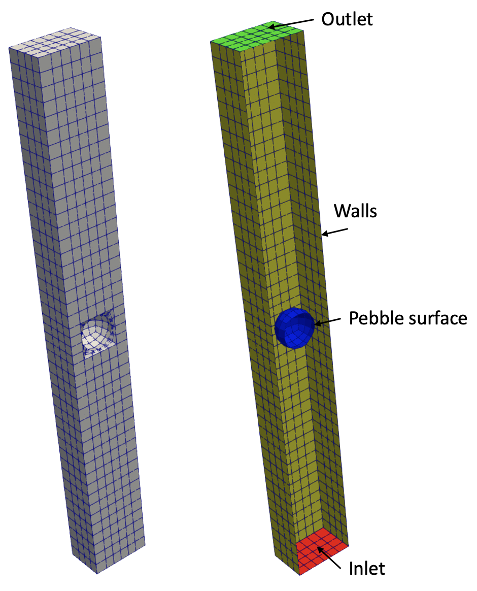
Figure 1: NekRS flow domain. Sidesets in the fluid domain are colored on the right.
NekRS shall solve for laminar flow over this pebble. Details on the problem specifications are given in Table 1. The inlet velocity is specified such that the Reynolds number is . The characteristic scale for the Reynolds number is chosen as the pebble diameter,
We will apply a uniform heat flux on the pebble surface. The pebble surface heat flux is selected to give a pebble power of approximately 893 W (giving a bulk fluid temperature rise of 50 K). In the conjugate heat transfer tutorials, this heat flux will later be replaced by coupling to MOOSE.
Table 1: Geometric and operating conditions for the single-pebble flow. Fluid properties correspond to water at standard atmosphere and temperature.
| Parameter | Value |
|---|---|
| Pebble diameter | 0.03 m |
| Box side length | 0.0506 m |
| Domain height | 0.4306 m |
| Fluid viscosity | 1e-3 Pa-s |
| Fluid density | 1000 kg/m |
| Fluid thermal conductivity | 0.6 W/m/K |
| Fluid volumetric specific heat | 4186 J/kg/K |
At a minimum, a NekRS model will constitute the following files:
pebble.re2: Mesh filepebble.par: High-level settings for the solver, boundary conditions, and the equations to solvepebble.udf: User-defined C++ functions for on-line postprocessing and model setuppebble.oudf: User-defined Open Concurrent Compute Abstraction (OCCA) kernels for boundary conditions and source terms
The default case file naming scheme used by NekRS is to use a common "casename" (in this case, we chose pebble), appended by the different file extensions which represents different parts of the input file setup. You can use a different naming scheme for the .re2, .udf, and .oudf files with settings in the .par file (discussed later).
Mesh (.re2 File)
NekRS uses a mesh in a custom .re2 format. The mesh must have hexahedral elements in either Hex8 (8-node hexahedral) or Hex20 (20-node hexahedral) forms. Hex20 is a second-order mesh format. The advantage of using a second-order format is evident for geometries with curves, like spheres or cylinders. As you refine to higher polynomial order, the mid-side quadrature points are moved to the curve surface to better capture the geometry. That said, exo2nek (discussed shortly) will automatically convert from tetrahedral and prism elements into hexahedral elements if you have a mesh starting with these other element types.
If you have a mesh in Exodus or Gmsh format, you can convert that mesh into .re2 format using tools that ship with Nek5000. To get these features, you will need to clone Nek5000 somewhere on your system and then build the exo2nek tool (for converting Exodus meshes) or the gmsh2nek tool (for converting Gmsh meshes).
git clone https://github.com/Nek5000/Nek5000.git
cd Nek5000/tools
./maketools exo2nek
Running the above will place a binary named exo2nek at Nek5000/bin/exo2nek. We recommend adding this to your PATH environment variable.
Now that you have exo2nek, we are ready to convert your mesh (pebble.exo) into .re2 format. This mesh is Hex8. Run the following:
exo2nek
Follow the on-screen prompts. For this case, we have:
1 fluid exo file, which is named
pebble.exo(you only need to providepebbleas the name)0 solid exo files (this is nonzero when NekRS is solving for both fluid and solid domains; in this example, we apply a surface heat flux, but are not actually solving for temperature in the solid with NekRS.)
0 periodic surface pairs (this is nonzero when applying periodic boundary conditions)
output file name is
pebble.re2(you only need to providepebbleas the output name)
This will create a mesh named pebble.re2. Alternatively, you can use the pebble.re2 file which is version-controlled in the repository.
NekRS is a spectral element code, which means that the solution in each element is represented as an -th order Lagrange polynomial (in each direction). An illustration for a 5th-order NekRS discretization is shown in Figure 2 for a 2-D element. Each red dot is a node (Gauss-Lobatto-Legendre (GLL) quadrature). When you create a mesh for NekRS, you do not see these GLL points in your starting Exodus/Gmsh mesh. Instead, they will be created when you launch NekRS (in other words, you do not need to create unique meshes if you want to run NekRS at different polynomial orders).
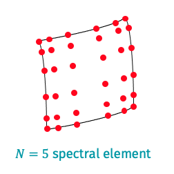
Figure 2: Nodal positions for a 5-th order polynomial solution.
.par File
The .par file is used to set up the high-level settings for the case. This file consists of blocks (in square brackets) and parameters.
userSections = CASEDATA

[OCCA]
  backend = CPU

[GENERAL]
  polynomialOrder = 3
  numSteps = 4000
  dt = targetCFL=2.0 + initial=1e-4
  checkpointInterval = 500
  scalars = temperature

[MESH]
  boundaryIDMap = 2, 3, 4, 5

[FLUID PRESSURE]
  residualTol = 1e-07

[FLUID VELOCITY]
  boundaryTypeMap = udfDirichlet, zeroNeumann, zeroDirichlet, zeroDirichletN/zeroNeumann
  residualTol = 1e-07
  rho = 1000.0
  viscosity = 1e-3

[SCALAR TEMPERATURE]
  boundaryTypeMap = udfDirichlet, zeroNeumann, udfNeumann, zeroNeumann
  residualTol = 1e-07
  transportCoeff = 4186000
  diffusionCoeff = 0.6

[CASEDATA]
  Re = 50
  D = 0.03
  inlet_T = 0
You can get a comprehensive list of all the syntax supported by running
$NEKRS_HOME/bin/nekrs --help par
OCCA block
This block is used to specify whether NekRS is running on CPU or GPU (and which vendor). For our case, we will run this on CPU so we set the backend as CPU.
GENERAL block
The [GENERAL] block describes the time stepping, simulation end control, and polynomial order. A NekRS output file is written every 500 time steps. The numSteps field indicate how many time steps to take. We will use a polynomial order of . We will begin with our first time step as seconds, but allow NekRS to adaptively increase this to get a target Courant-Friedrichs-Lewy (CFL) number of 2.0.
MESH block
The [MESH] block in this example is used to list the ordering of sidesets as they pertain to the ordering of the boundary conditions in the boundaryTypeMap parameters in other blocks. In other words, the first boundary condition given in these lists corresponds to mesh sideset 2, and so on.
FLUID VELOCITY, FLUID PRESSURE, SCALAR TEMPERATURE blocks
Next, the [FLUID VELOCITY] and [FLUID PRESSURE] blocks describe the solution of the pressure Poisson equation and velocity Helmholtz equations. The [SCALAR TEMPERATURE] block describes the solution of the energy equation. NekRS can also solve for an arbitrary number of coupled passive scalars, which would be represented using [SCALAR FOO] blocks, where FOO would be replaced with a string describing the name of the scalar (e.g. [SCALAR K] for the turbulent kinetic energy when using a Reynolds Averaged Navier-Stokes (RANS) model).
In these blocks, residualTol is used to indicate the solver tolerance. Here, you also specify the type of boundary conditions to apply to each sideset (you only specify boundary conditions in the [FLUID VELOCITY] and [SCALAR FOO] blocks, because the pressure and velocity solves are really indicating together a solution to the momentum conservation equation). The boundaryTypeMap is used to specify the mapping of boundary IDs to types of boundary conditions. NekRS uses character strings to refer to the type of boundary condition; full information can be found on the NekRS website.
Some of the common boundary condition strings are shown in Table 2. When you specify these boundary conditions, the boundary conditions requiring user information (e.g. udfDirichlet, udfNeumann, and udfRobin) will trigger the requirement for you to provide functions by the same name in the .oudf file.
Table 2: Common boundary conditions in NekRS
| Meaning | How to set in .par File | Function name in .oudf File |
|---|---|---|
udfDirichlet | Dirichlet velocity or temperature | udfDirichlet |
zeroDirichlet | Zero Dirichlet value (e.g. no-slip wall) | — |
zeroNeumann | Outflow velocity + Dirichlet pressure, insulated | — |
zeroDirichletX/zeroNeumann | symmetry in the -direction | — |
zeroDirichletY/zeroNeumann | symmetry in the -direction | — |
zeroDirichletZ/zeroNeumann | symmetry in the -direction | — |
zeroDirichletN/zeroNeumann | general symmetry boundary | — |
When you populate boundaryTypeMap in the input file, you simply list the character string for your desired boundary condition in the same order as the sidesets. If your sidesets are already ordered sequentially, nothing else needs to be done. Otherwise, you need to provide the boundaryIDMap field in the [MESH] block as described earlier.
In each of the equation blocks, different parameter names are used to indicate the properties which are multiplying the time and diffusive terms.
Names of parameters for properties in each block
| Block | Coefficient on time derivative | Coefficient on diffusive term |
|---|---|---|
[FLUID VELOCITY] | rho | viscosity| |
[SCALAR FOO] | transportCoeff | diffusionCoeff |
For convenience, NekRS allows you to pull parameters from the .par file elsewhere throughout your case files. In order to streamline the model setup, you can add any number of user-defined blocks by setting the userSections parameter and then providing those blocks. In this example, we illustrate this for a [CASEDATA] block where we define local variables which we arbitrarily name name Re, D, and inlet_T which we'll use in our boundary and initial conditions.
.udf File
The .udf file contains additional C++ code which is typically used for setting initial conditions and postprocessing. This file at a minimum must contain 2 functions (they can be empty):
UDF_Setupis called on initialization time, and is typically where initial conditions are appliedUDF_ExecuteStepis called once on each time step, and is typically where postprocessing is applied
static dfloat inlet_v;
static dfloat inlet_T;
static dfloat Re;
static dfloat D;
static dfloat mu;
static dfloat rho;

#ifdef __okl__

#include "pebble.oudf"

#endif

void UDF_Setup0(MPI_Comm comm, setupAide &options)
{
  // get parameters from .par file
  platform->par->extract("casedata", "D", D);
  platform->par->extract("casedata", "Re", Re);
  platform->par->extract("casedata", "inlet_T", inlet_T);
  platform->options.getArgs("FLUID VISCOSITY", mu);
  platform->options.getArgs("FLUID DENSITY", rho);
}

void UDF_LoadKernels(deviceKernelProperties & kernelInfo)
{
  // send parameter to device
  inlet_v = Re * mu / D / rho;
  kernelInfo.define("p_inlet_v") = inlet_v;
  kernelInfo.define("p_inlet_T") = inlet_T;
}

void UDF_Setup()
{
  auto mesh = nrs->meshV;

  // arbitrary arrays on the host where we will fill some initial data
  std::vector<dfloat> U(nrs->fluid->fieldOffsetSum, 0.0);
  std::vector<dfloat> temp(mesh->Nlocal, 0.0);

  for (int n = 0; n < mesh->Nlocal; ++n)
  {
    U[n + 0 * nrs->fieldOffset] = 0.0; // x-velocity
    U[n + 1 * nrs->fieldOffset] = 0.0; // y-velocity
    U[n + 2 * nrs->fieldOffset] = inlet_v; // z-velocity

    temp[n] = inlet_T; // temperature
  }

  // copy host data into the device data
  nrs->fluid->o_U.copyFrom(U.data(), U.size());
  nrs->scalar->o_solution("temperature").copyFrom(temp.data(), temp.size());
}

void UDF_ExecuteStep(double time, int tstep)
{
}
Here, we use the UDF_Setup function to set initial conditions (to the same values we applied as our inlet boundary conditions). Because NekRS is a GPU code, most data structures only exist on the device. Therefore, in order to set initial conditions, we declare some empty vectors of the appropriate lengths for velocity and temperature, fill them with our desired initial conditions, and then copy them into the device.
NekRS stores the various solution components on the device as
nrs->fluid->o_Uis velocity (all three components are packed one after another, with each "slice" of lengthnrs->fieldOffset)nrs->fluid->o_Pis pressurenrs->scalar->o_solution("foo")is the passive scalar namedFOOin the.parfile
By default, initial conditions are taken to be zero unless otherwise specified; because we did not specify an initial condition for pressure, this means our initial pressure will be zero in this problem.
Our problem only has one passive scalar (temperature). You will have additional passive scalars if doing RANS modeling (e.g. and would be passive scalars) or if you have additional conservation equations for mass transport, etc. We apply the initial condition by looping over all the degrees of freedom on the present MPI rank.
Our .udf file has two additional (optional) functions which we use to set up other aspects of the simulation. The UDF_Setup0 function is where we extract parameters from the .par file. We fetch the values we provided in the [CASEDATA] block, as well as the viscosity and density we gave in the [FLUID VELOCITY] block.
Finally, the UDF_LoadKernels function is where we can load GPU kernels and send parameters to the device. The kernelInfo lines in particular are sending the inlet_v and inlet_T values from host to device, so that we can later access them from the .oudf file. It is customary when sending a value to device to prepend p_ to the name, to help with clarity.
.oudf File
When you define the boundary condition types in the .par file, you also need to set the values of those boundary conditions (the non-trivial ones) n the .oudf file. The names of these functions are pre-defined by NekRS, and are paired up to the character strings you set earlier. These function names are shown in Table 2 in the .oudf column. Note that a --- indicates that no user-defined kernels are necessary to define that boundary condition (i.e. NekRS already has all the info it needs to apply a zero-Dirichlet boundary condition - it just sets the solution to zero).
For each of these functions, the bcData struct contains all information about the current boundary that is "calling" the function:
bc->idis the boundary IDbc->uxFluidis the -velocitybc->uyFluidis the -velocitybc->uzFluidis the -velocitybc->sScalaris the scalar solution at the present quadrature point; if there are multiple scalars, this should be placed inside anif (isField("scalar foo"))to ensure you only set the value of theFOOscalar.bc->fluxScalaris the flux of the scalar at the present quadrature point; if there are multiple scalars, this should be placed inside anif (isField("scalar foo"))to ensure you only the the flux of theFOOscalar.bc->idxVolis the index corresponding to the current quadrature point
void udfDirichlet(bcData *bc)
{
  if (isField("fluid velocity"))
  {
    bc->uxFluid = 0.0; // x-velocity
    bc->uyFluid = 0.0; // y-velocity
    bc->uzFluid = p_inlet_v; // z-velocity
  }

  if (isField("scalar temperature"))
    bc->sScalar = p_inlet_T; // temperature
}

void udfNeumann(bcData *bc)
{
  // power divided by sphere surface area
  bc->fluxScalar = 315892;
}
.usr File
NekRS is under rapid development, and many features from Nek5000 are currently being ported over to NekRS. To access those Fortran-based features, you can optionally include a .usr file, which contains funtions for setting initial conditions, modifying the mesh, etc. We do not need this file for this case, so we will defer to a later tutorial to demonstrate it.
Execution and Postprocessing
When you compile Cardinal, you automatically also get a standalone NekRS executable. You can run the NekRS case with
$NEKRS_HOME/bin/nrsmpi pebble 4
where pebble is the case name and 4 is the number of MPI ranks you would like to use. Note that NekRS does not use any shared memory parallelism (e.g. OpenMP). Running this case will produce NekRS output files named pebble0.f<n>, where <n> is a 5-digit integer indicating the output file number (i.e. they will be sequentially-ordered based on when you told NekRS to write output files).
These files (referred to as "field" files) need to be accompanied by a small "configuration" file in order to load into Paraview. This file is automatically generated by NekRS, and will be named pebble.nek5000 for this case. If we open this file, we see it has very simple contents:
filetemplate: pebble%01d.f%05d
firsttimestep: 0
numtimesteps: 8
This file tells Paraview how many time steps there are to load and the naming pattern for those files. To open the NekRS output files, you then need to open the pebble.nek5000 file.
To open the files in Paraview or Visit, you must also have co-located with the pebble.nek5000 files your actual output files from NekRS (e.g. the pebble0.f<n> files).
First, let's take a look at the mesh to get a better sense for how NekRS stores data in its output files. Figure 3 shows a zoomed-in view near the pebble surface. As you can see, this mesh displays the GLL quadrature points. Outlined in red is a single element in our starting Exodus mesh (pebble.exo); the lines inside each element are connecting the nodes.
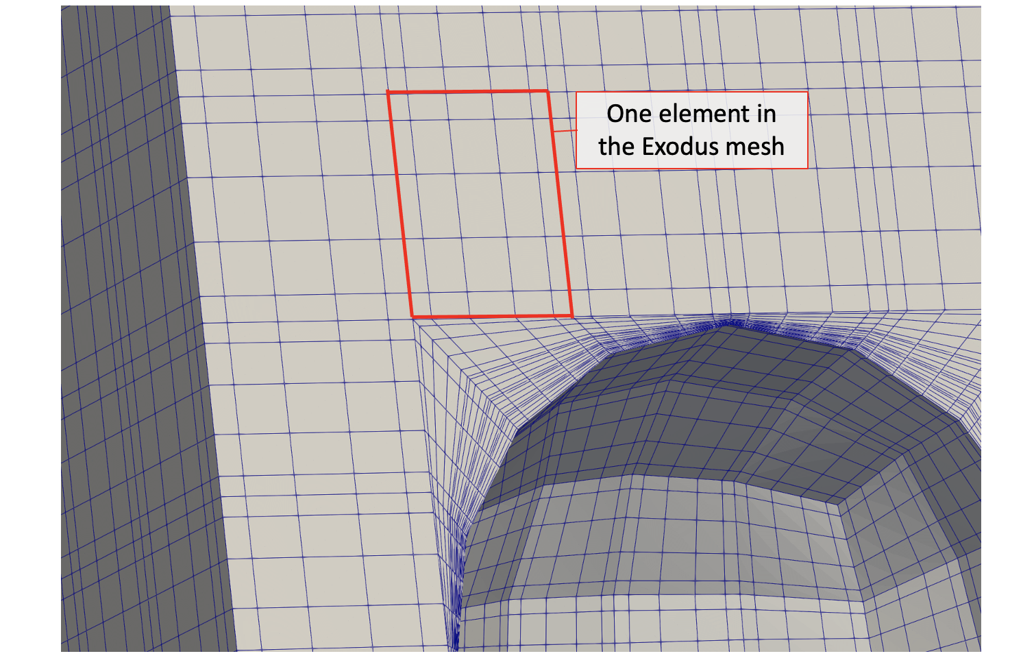
Figure 3: NekRS spectral mesh, for polynomial order 5
Note that the pebble surface is "faceted" in the same way as our starting Exodus mesh. This is the case because we used a first-order Hex8 mesh. Next, Figure 4 shows the velocity, pressure, and temperature predicted by NekRS.
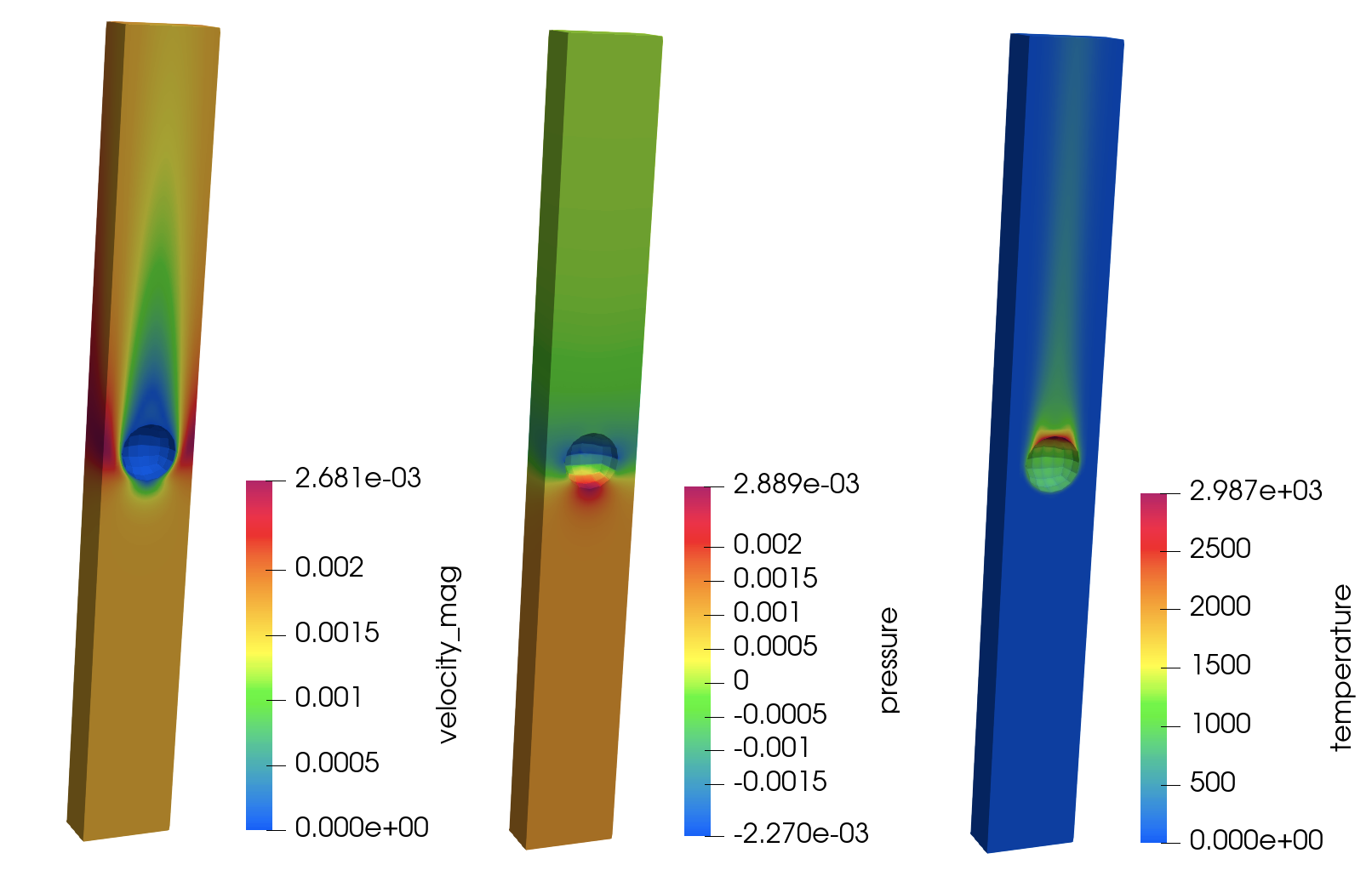
Figure 4: NekRS predicted velocity, pressure, and temperature for laminar flow
Hex8 vs Hex20
To appreciate the difference between Hex8 and Hex20 meshes, Figure 5 shows the GLL points which would be used by NekRS if our input mesh was instead in Hex20 format. As you can see, the mid-side nodes follow the curvature of the sphere because the (single) mid-side node in our starting Hex20 mesh "knows about" the curve in the mesh at this point.
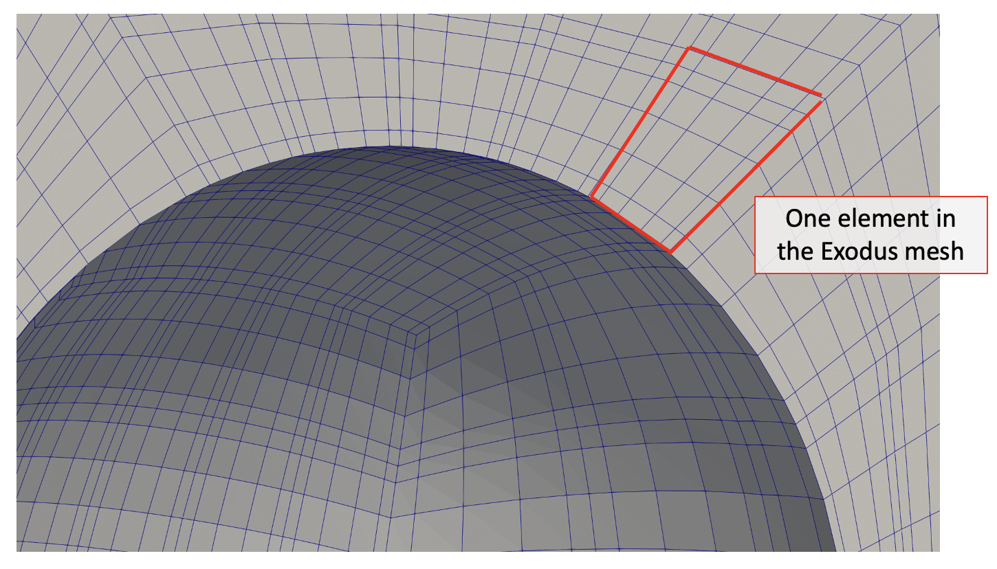
Figure 5: NekRS mesh for polynomial order 5 when using a Hex20 input mesh