Moving Cylinder (Low-Mach)
The mv_cyl case verifies the low-Mach and moving-mesh capabilities in NekRS using a moving piston in a quasi-two-dimensional domain. The piston is located at , while a stationary wall is located at . The domain has width , and symmetry boundary conditions are imposed at .
Governing equations
Under the ideal-gas assumption, the nondimensional low-Mach governing equations are
(1)Here, is the thermal divergence, is the thermodynamic pressure, is the hydrodynamic pressure, is the ratio of specific heats, is the strain-rate tensor, and is the identity tensor. The Reynolds and Péclet numbers are denoted by and , respectively.
Analytical solution
The piston is prescribed a sinusoidal velocity,
(2)where is the piston velocity amplitude. The flow remains isentropic, and the analytical solution is
(3)Here, is the piston location, is the initial domain volume, is the instantaneous domain volume, is the initial thermodynamic pressure, is the piston surface area, and is the spatially averaged temperature.
Verification criterion
The tests are qualified by evaluating the absolute errors in at a specified time. Because these quantities are spatially uniform, the case also verifies the expected temporal convergence rate.
For the various tests, the mesh velocity is either prescribed analytically as,
(4)or the mesh motion is computed using the elasticity solver with the piston velocity prescribed as a Dirichlet boundary condition. The resulting temporal convergence is presented below. The tests are organized into various solver modes, as follows:
Mode 1
This solver mode tests:
Low-Mach solver.
Passive scalar solver.
Prescribed moving mesh.
Errors are computed at and are shown in Figure 1.
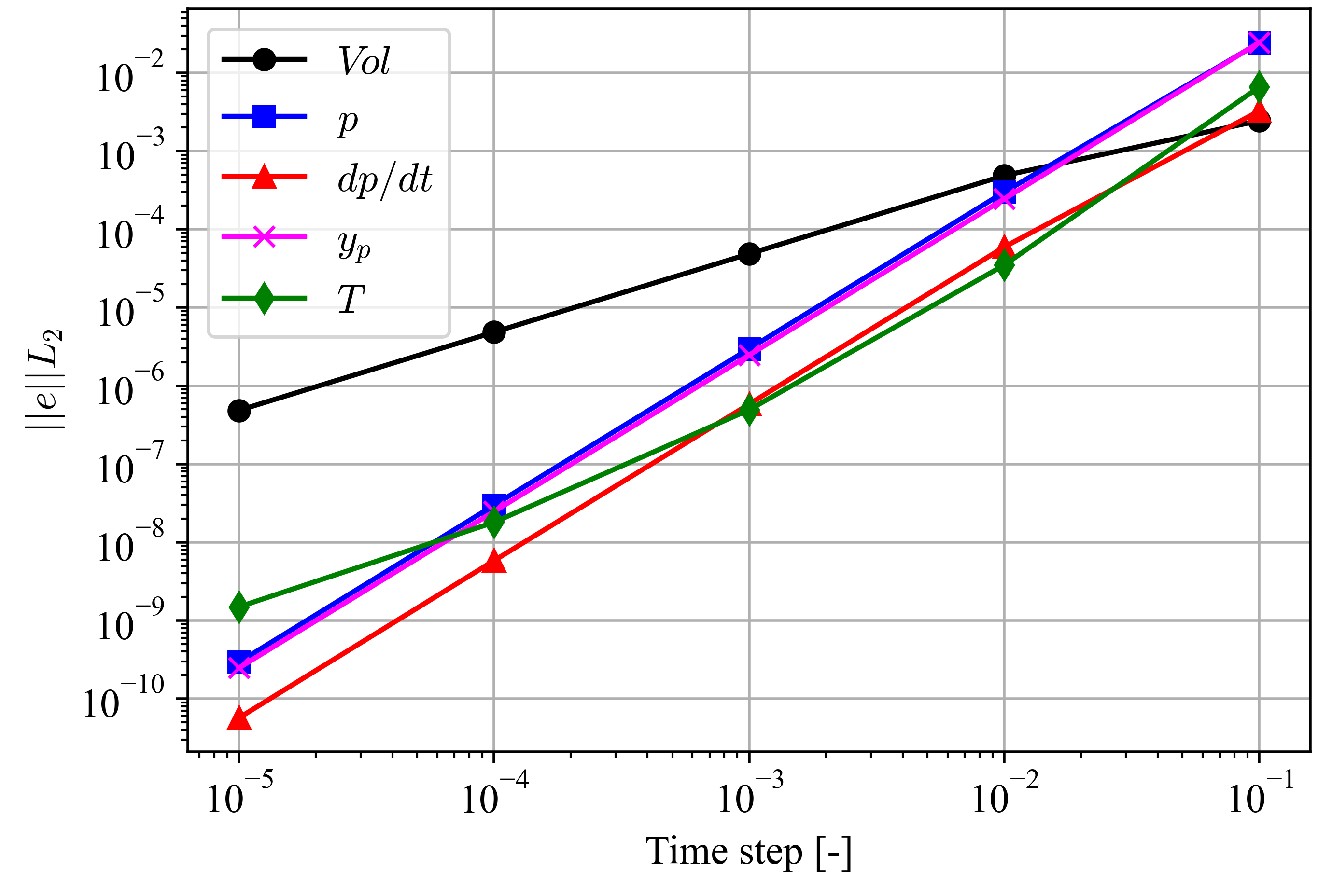
Figure 1: Temporal convergence for the mv_cyl case using solver mode 1.
Mode 2
This solver mode tests:
All capabilities exercised in solver mode 1.
Characteristic subcycling.
Errors are computed at and are shown in Figure 2.
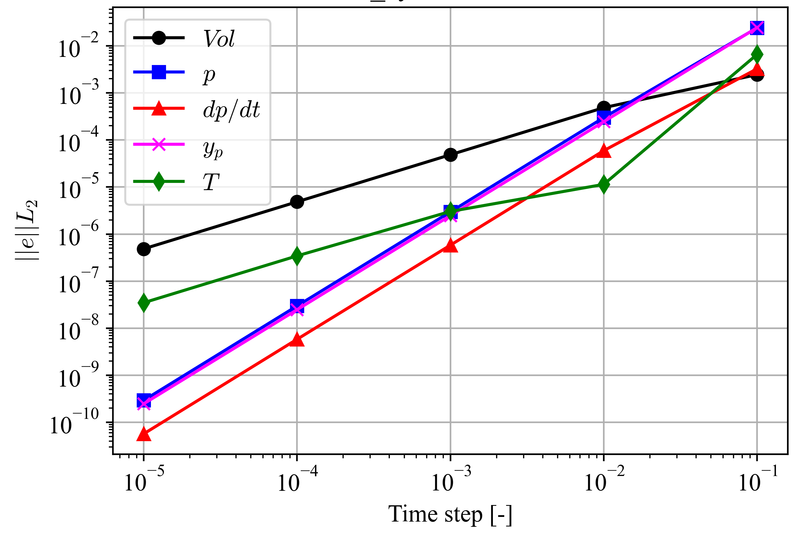
Figure 2: Temporal convergence for the mv_cyl case using solver mode 2.
Mode 3
This solver mode tests:
All capabilities exercised in solver mode 2.
Elasticity mesh solver.
Mesh projection.
Errors are computed at and are shown in Figure 3.
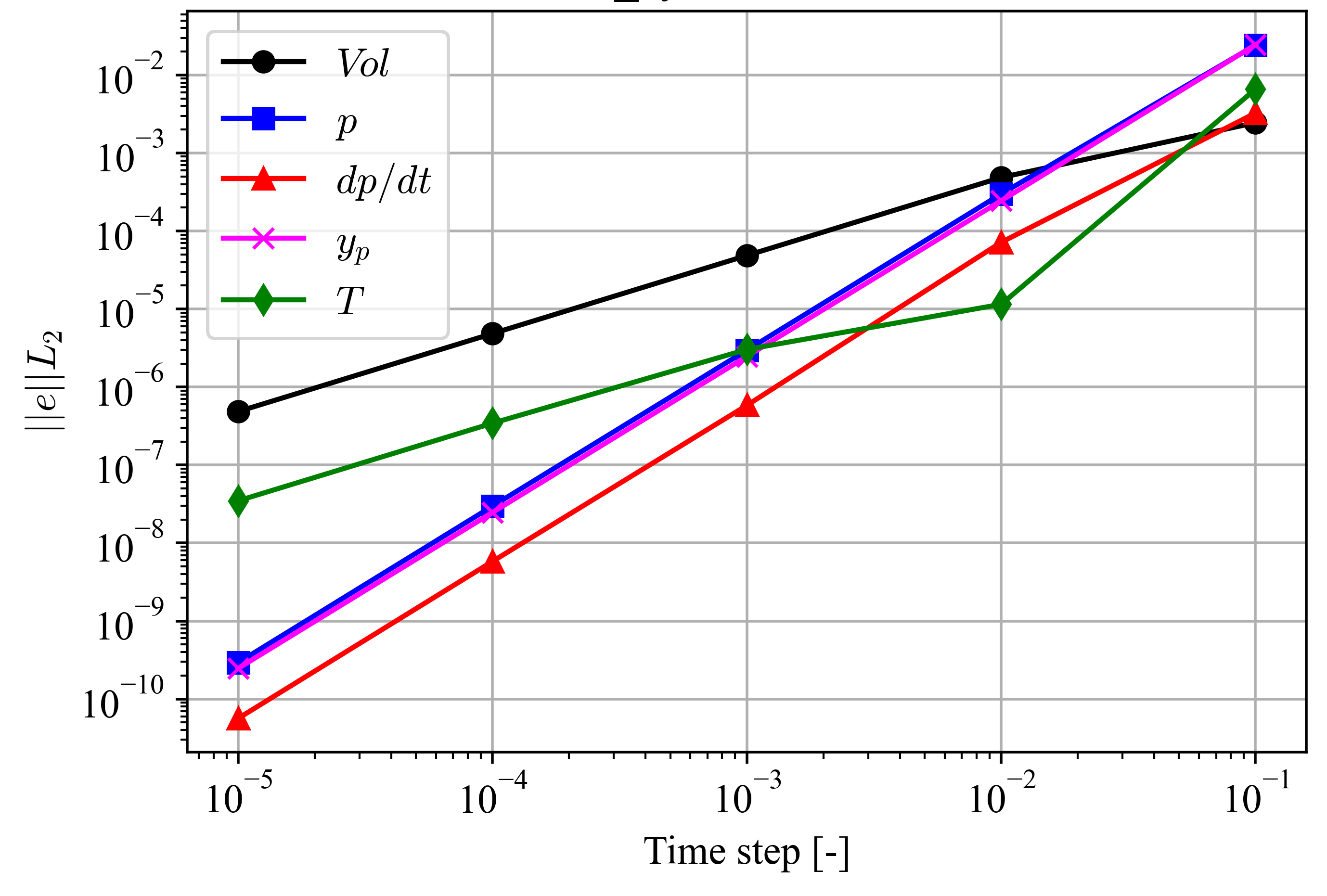
Figure 3: Temporal convergence for the mv_cyl case using solver mode 3.
Mode 5
This solver mode verifies the capabilities of solver mode 1 on an unaligned mesh. Errors are computed at and are shown in Figure 4.
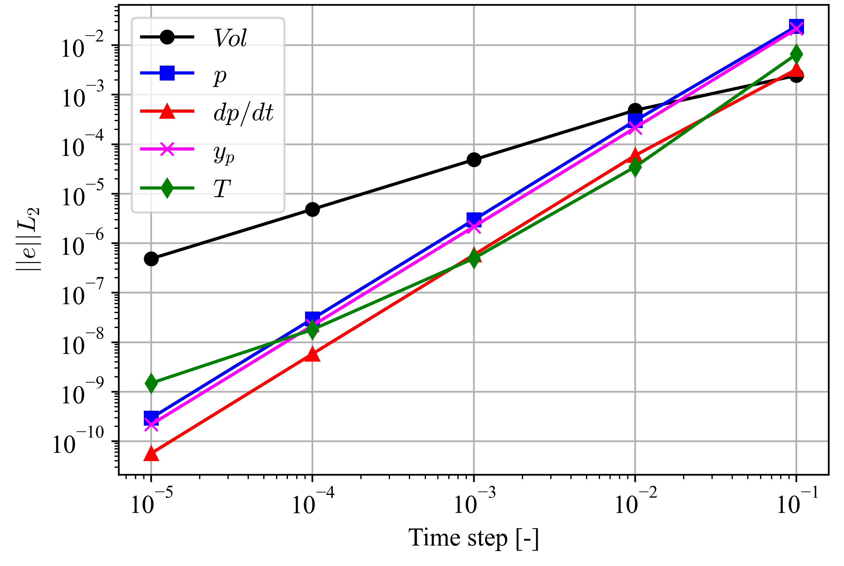
Figure 4: Temporal convergence for the mv_cyl case using solver mode 5.
Mode 6
This solver mode verifies the capabilities of solver mode 3 on an unaligned mesh. Errors are computed at and are shown in Figure 5.
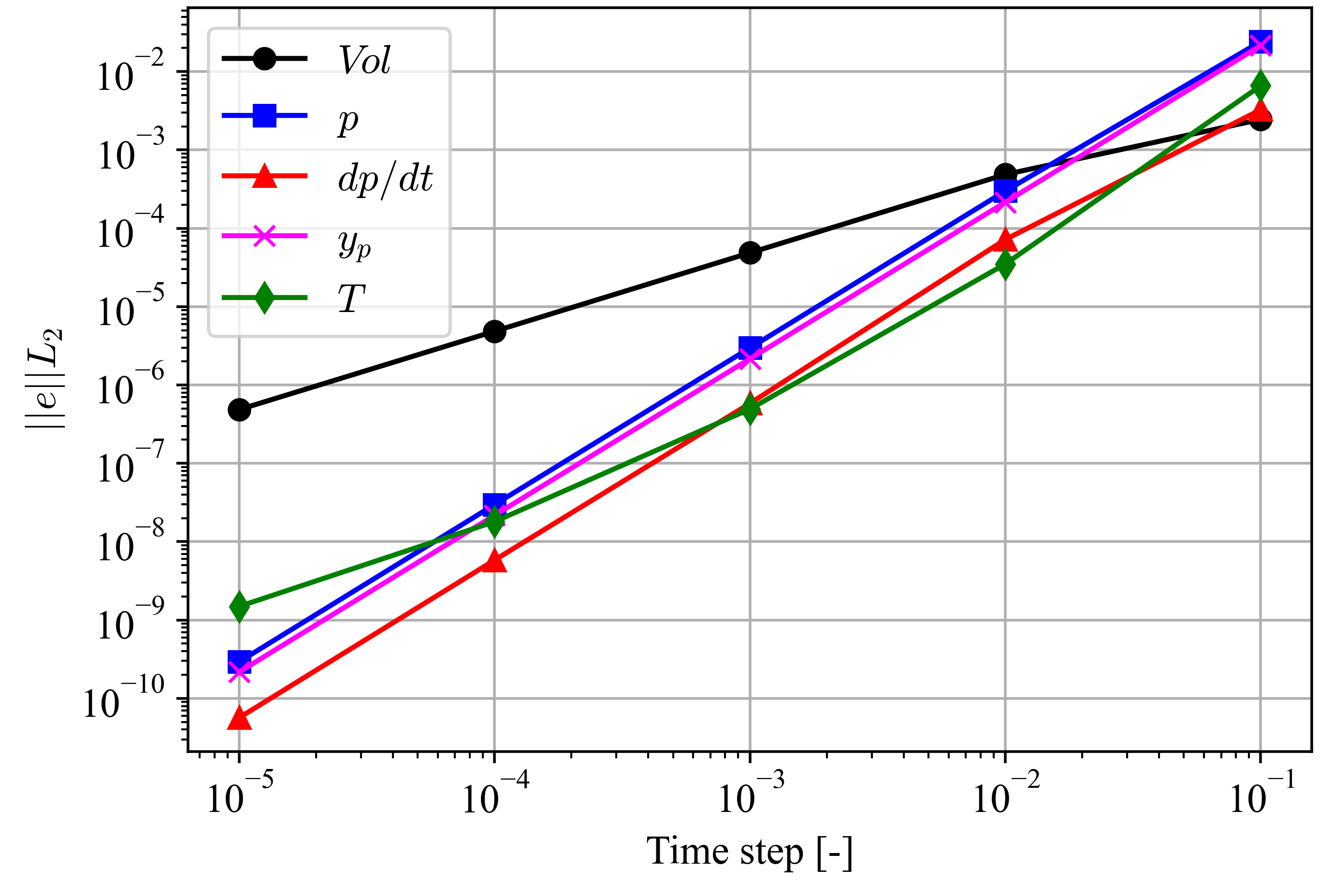
Figure 5: Temporal convergence for the mv_cyl case using solver mode 6.