BISON User Workshop
Implicit, parallel, fully-coupled nuclear fuel performance analysis
Computational Mechanics and Materials Department
Idaho National Laboratory
BISON Team Members
Rich Williamson
(Richard.Williamson@inl.gov)Steve Novascone
(Stephen.Novascone@inl.gov)Jason Hales
(Jason.Hales@inl.gov)Ben Spencer
(Benjamin.Spencer@inl.gov)Kyle Gamble
(Kyle.Gamble@inl.gov)Gyanender Singh
(Gyanender.Singh@inl.gov)
Stephanie Pitts
(Stephanie.Pitts@inl.gov)Adam Zabriskie
(Adam.Zabriskie@inl.gov)Aysenur Toptan
(Aysenur.Toptan@inl.gov)Wen Jiang
(Wen.Jiang@inl.gov)Pierre-Clément Simon
(pierreclement.simon@inl.gov)Wenfeng Liu
(Wliu@Structint.com)Christopher Matthews
(cmatthews@lanl.gov)
BISON Overview
Fuel Behavior: Introduction
At beginning of life, a fuel element is quite simple...
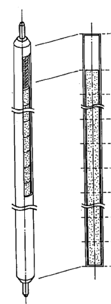
Nakajima et al., Nuc. Eng. Des., 148, 41 (1994)
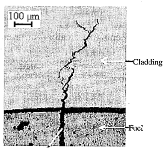
but irradiation brings about substantial complexity...
Michel et al., Eng. Frac. Mech., 75, 3581 (2008)
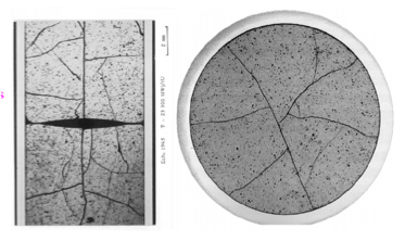
Fuel Fracture
Olander, p. 584 (1978)
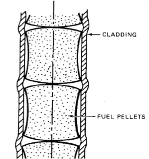
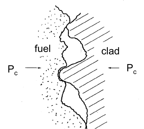
Multidimensional Contact
and Deformation
Olander, p. 584 (1978)
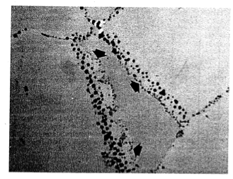
Fission Gas
Bentejac et al., PCI Seminar (2004)
Stress Corrosion
Cracking Cladding
Failure
Fuel Behavior Modeling: Coupled Multiphysics
Multiphysics
Fully coupled nonlinear thermo-mechanics
Multiple species diffusion
Neutronics
Thermal-hydraulics
Chemistry
Multi-space scale
Important physics at the atomistic and micro-structural levels
Practical engineering simulations require the continuum level
Multi-time scale
Steady operation ( week)
Power ramps/accidents
( s)

BISON - Nuclear Fuel Performance Analysis
BISON is a nuclear fuel performance analysis tool. It is used primarily for analysis of fuel but has also been used to model TRISO fuel, both rod and plate metal fuel, and accident tolerant fuel. BISON is built on top of MOOSE.
BISON is implicit
Large time steps
BISON runs in parallel
Runs naturally on one or many processors
BISON is fully coupled
No operator splitting or staggered scheme necessary
All unknowns are solved for simultaneously
BISON is under development; there is still much to do
Fission gas release model continues to improve
Contact can be a challenge; friction needs improvement
Automatic time-stepping needs improvement
Documentation and validation is evolving
BISON's Relationship to MOOSE
Code too specific for MOOSE but useful for multiple applications is collected in libraries.
BISON depends on:
MOOSE modules (solid mechanics, fluid dynamics, etc.) depends on:
MOOSE (multiphysics application framework) depends on:
libMesh (numerical PDE solution framework out of UT Austin) depends on:
PETSc, Exodus II, MPI, etc.
BISON LWR Capabilities
General Capabilities
3D, 2D-RZ, 1D fully coupled thermo-mechanics
Large deformations
Parallel
Meso-scale informed
Oxide Fuel Behavior
Temperature/burnup/porosity dependent material properties
Volumetric heat generation
Thermal and fission product swelling, and densification strains
Thermal and irradiation creep
Fuel fracture via relocation and smeared cracking
Fission gas release (2 stages)
transient release
grain growth/sweeping
athermal release
Temperature
Gap/Plenum Behavior
Gap heat transfer with
Mechanical contact
Plenum pressure as a function of:
evolving gas volume (from mechanics)
gas mixture (FGR)
gas temperature approximation
Cladding Behavior
Thermal and irradiation creep
Thermal expansion
Irradiation growth
Plasticity
Hydride damage
Coolant Channel
Closed channel thermal hydraulics with heat transfer coefficients
BISON Example - Axisymmetric LWR Fuel Rodlet
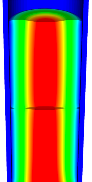
BISON Results - Axisymmetric LWR Fuel Rodlet
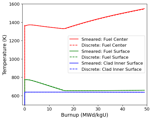
Thermal expansion, fuel densification, clad creep-down, fission gas release, contact, and burnup dependent fuel thermal conductivity all affect fuel temperatures
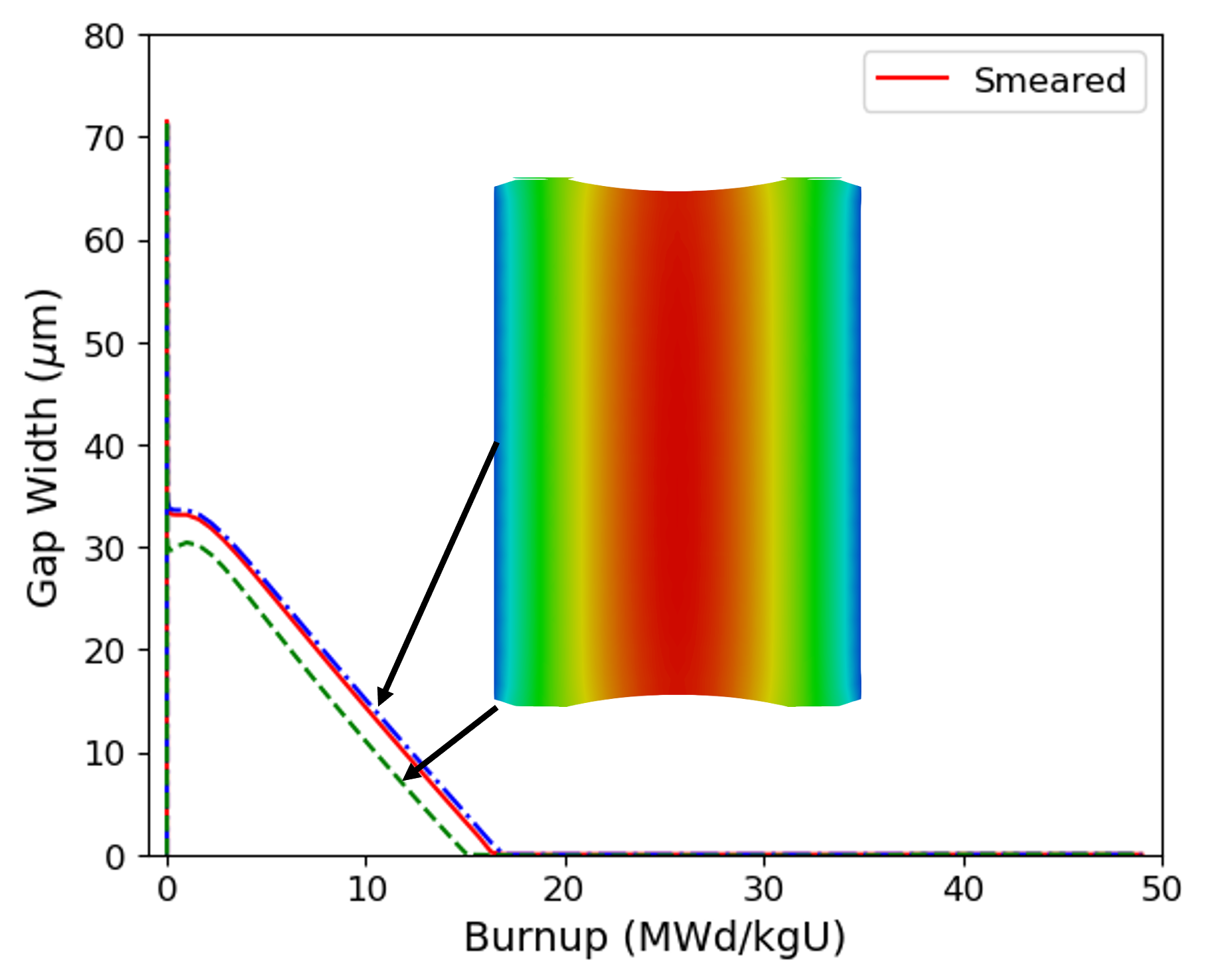
Hourglass shape of pellets is evident in gap closure histories
BISON Results - Axisymmetric LWR Fuel Rodlet
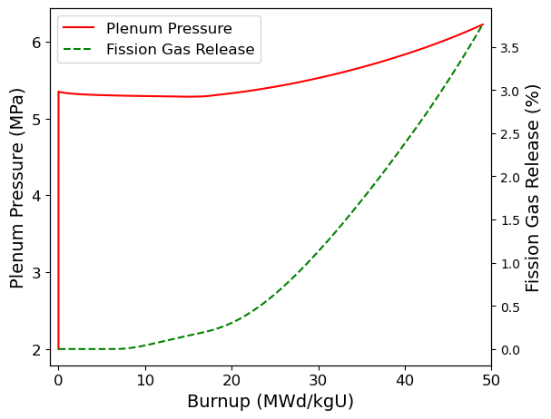
Fission gas release begins at a burnup of 10 MWd/kgU
Hourglass shape of pellets creates ridges in clad during PCMI
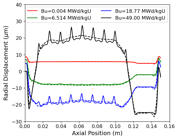
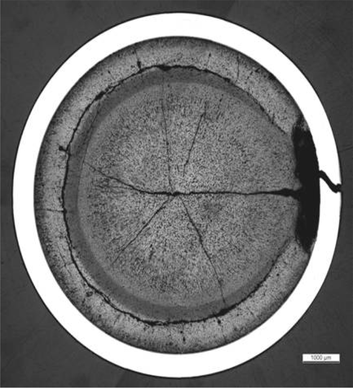
BISON Example - Missing Pellet Surface
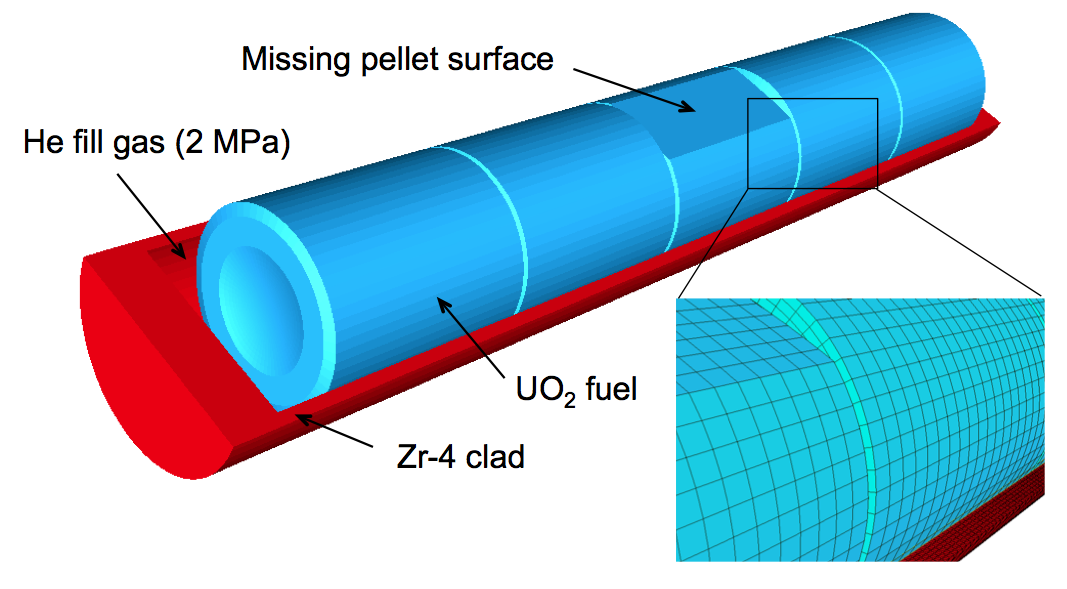
High-resolution 3D calculation (25,000 elements, 1.1 dof) run on 120 processors
Simulation starting from a fresh fuel state with a typical power history, followed by a late-life power ramp
BISON Results - Missing Pellet Surface
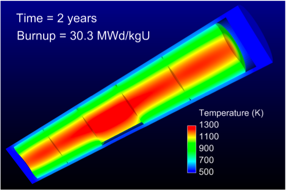
Fuel Temperature
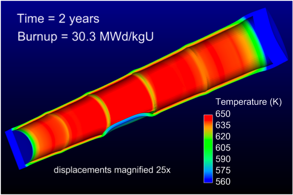
Clad Temperature
Missing pellet surface has a very significant effect on the temperature and stress state in the rod
Model can be used to examine source of rod failures
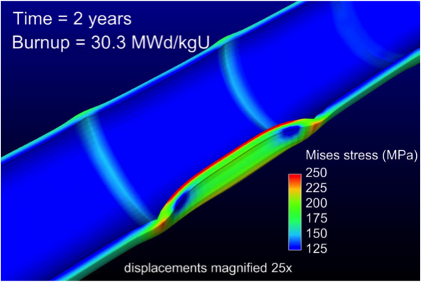
Clad Stress
BISON Coated-Particle Fuel Capabilities
General Capabilities
3D, 2D-RZ, 1D fully coupled thermomechanics with species diffusion
Large deformation
Elasticity with thermal expansion
Steady and transient
Massively parallel
Fuel Kernel
Temperature, burnup, porosity dependent conductivity
Solid and gaseous fission product swelling
Densification
Thermal/irradiation creep
Fission gas release
CO production
Radioactive decay
Tangential Stress
Gap Behavior
Gap heat transfer with
Gap mass transfer
Mechanical contact
Plenum pressure as a function of:
evolving gas volume (from mechanics)
gas mixture (FGR and CO)
gas temperature approximation
Silicon Carbide
Irradiation creep
Pyrolytic Carbon
Anisotropic irradiation-induced strain
Irradiation creep
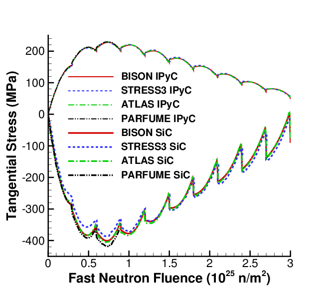
BISON Results - TRISO Particle
Validated against PARFUME, ATLAS, STRESS3
Code comparisons are excellent
Run times of 1 s are typical
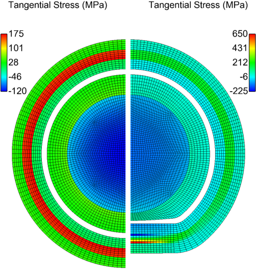
PBR cyclic particle temperature
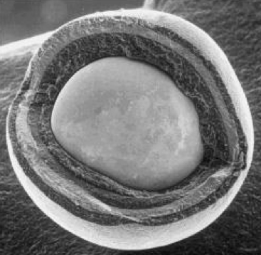
Aspherical particles are common
Raises peak tensile stress by 4x
Runs in a few minutes (8 procs)
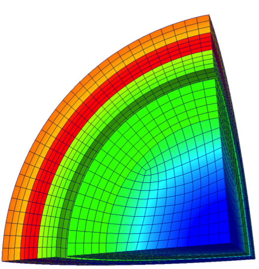
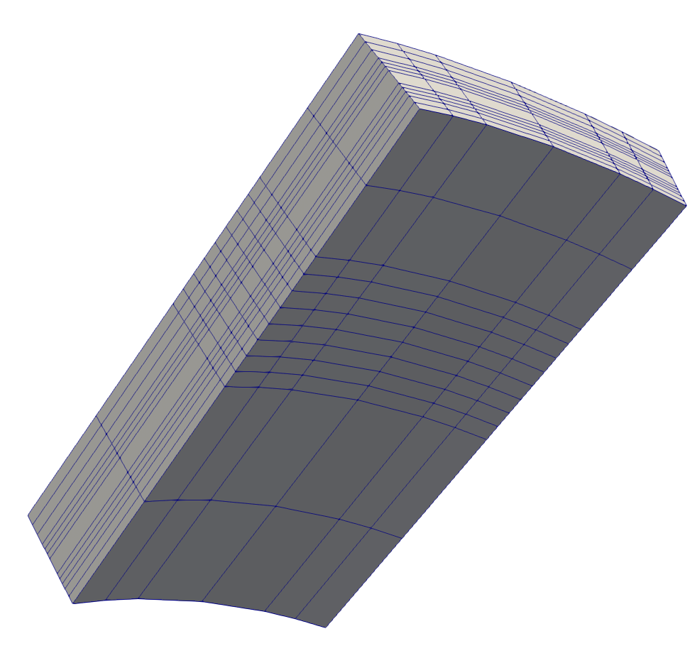
BISON Results - 3D Simulation of Thinned SiC Layer
Localized SiC thinning due to soot inclusions or fission product interaction
3D capability demonstrated on eighth particle with random thinning
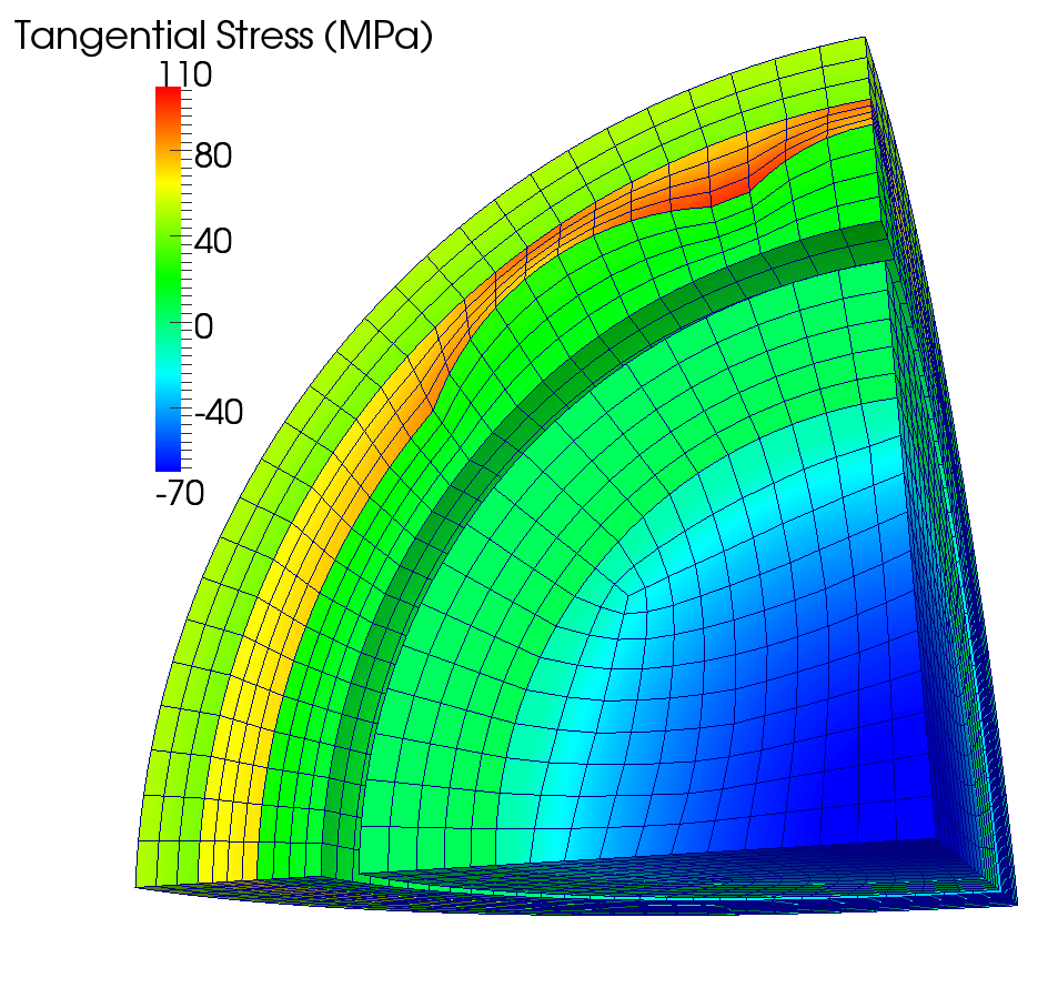
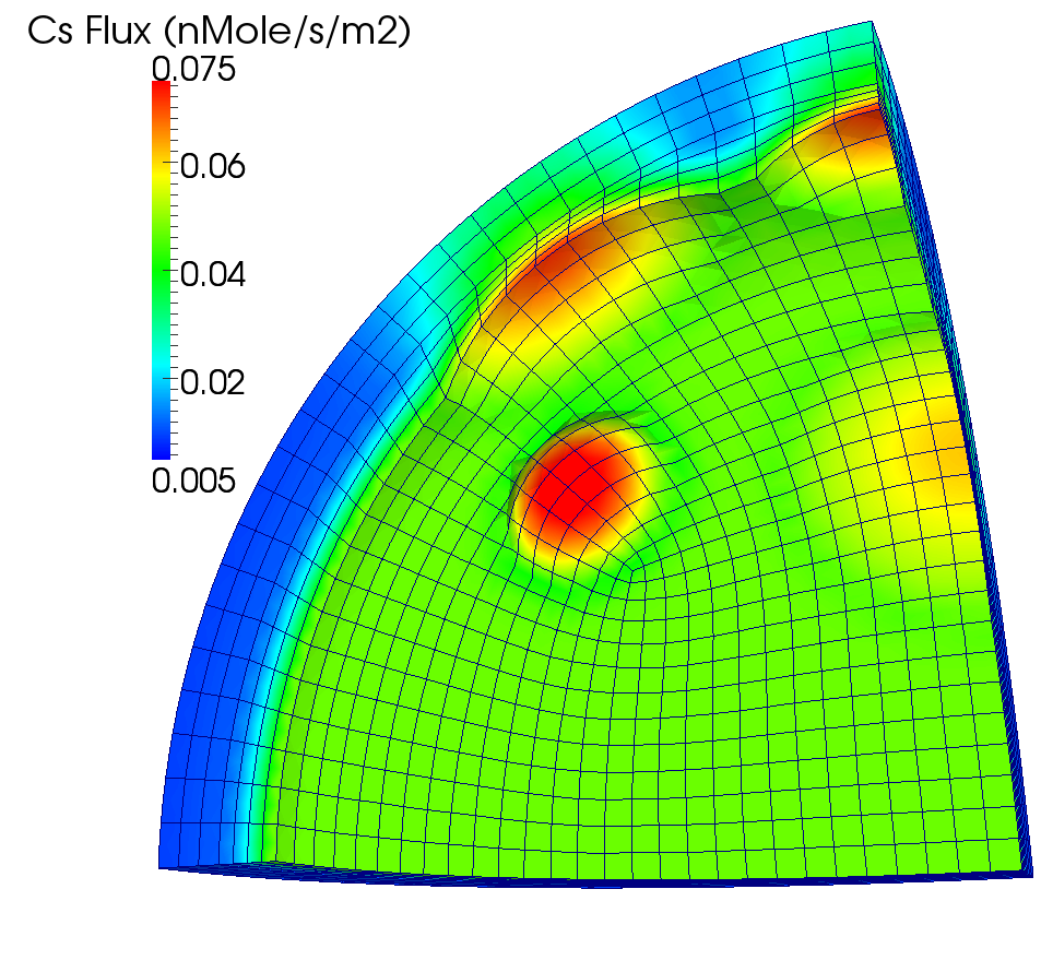
Significantly higher tensile stress and cesium release; impossible to predict with state-of-the-art 1D or 2D analyses
Typical run times of a few hours on 8 procs
BISON Documentation
Documentation Overview
The documentation for BISON is developed in Markdown (.md) and viewed in an internet browser.
The documentation includes:
Getting Started Instructions
Examples
General Theory
BISON and MOOSE Code Reference Manuals
Software Quality Documents
Verification and Validation
Frequently Asked Questions
Contact Us
Accessing the Documentation
There are three ways to access the documentation:
A publicly available version is located at https://mooseframework.org/bison/ and is built from the latest version of the master (stable) branch of BISON.
An internally available version is located at https://bison-dev.hpc.inl.gov/site/ and is built from the latest version of the master (stable) branch of BISON. HPC login credentials are required.
A version can be built directly in your local copy of the repository and will include any local modifications and additions to the documentation.
cd bison/doc/
./moosedocs.py build --serve
Paste the provided address (https://127.0.0.1:8000) into a browser.
Git, Submodules, and Updates
Git
Git is a version control software.
Everyone will use Git to update BISON.
Contributors to BISON will also use Git to prepare merge requests.
Git is a very powerful tool. As such, if you want to learn it, download the free book Pro Git.
Check out the first three chapters at least.
Terminology
repository (repo for short) is where you clone from. We have two:
idaholab is the official location for BISON.
your_user_name is the location of your "fork" of BISON.
fork is a repo created by you from idaholab/bison.
Users do not need to create a fork.
Contributors must create a fork.
Once a fork is created, it is its own entity separate from idaholab/bison.
clone is how you copy what is in a repo to a directory.
origin is a name for the repo you originally cloned from.
upstream is a name or alias set for idaholab/bison repo.
NOTE: If you originally cloned from idaholab, then you don't need an upstream. "origin" is idaholab/bison.
Git Environment
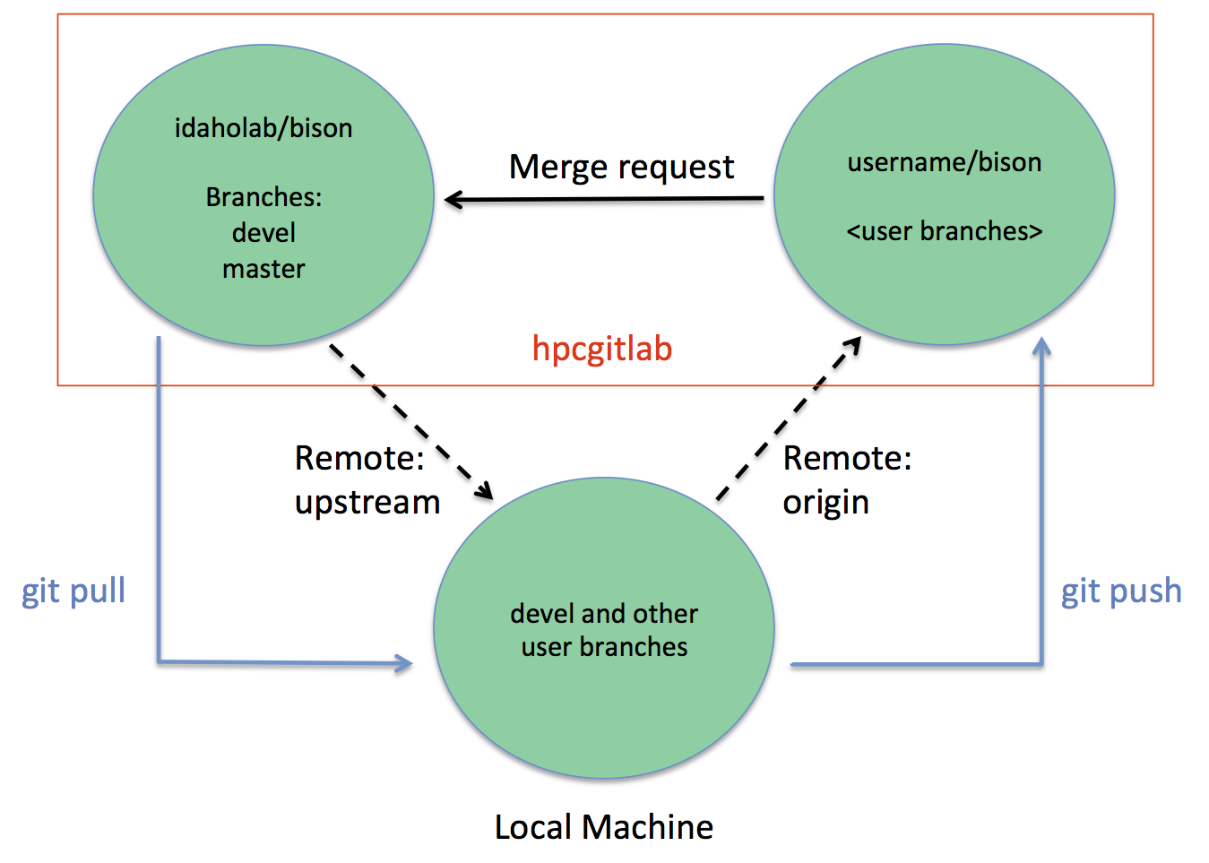
This is a pictorial diagram of our Git environment. In this diagram, local machine represents either a physical, local machine or the HPC. The two upper circles represent space on https://github.inl.gov. The dotted arrows upstream and origin represent Git remote names.
Git Repository Overview
A Git repository has more than just files in it. It has history, too!
Each "commit" adds a page to that history.
Use
git logto look at the identifier, author, date, and description of commits.A commit identifier is a SHA-1 hash of the contents of that commit and is unique to that commit. Example:
521747298a3790fde1710f3aa2d03b55020575aaUsually, only the first 7 digits is needed to identify a commit.
History can branch out and merge back together.
Your location is the commit you are on.
Branches are a convenient way to keep track of commits that link together.
Git Forks
Contributors (and some users) of BISON will have forks of BISON.
Recall that forks become their own repository after creation.
A fork does not automatically receive or send information to the original repository.
You own your fork and can do anything there without fear of ruining the official BISON repository (idaholab/bison).
You, the owner of the fork, must manually receive or send (contribute) from or to the original repository.
Contributing code requires review and will be covered later.
Forks allow for "spiderweb-like" development and collaboration.
Forks may be added as remote repositories with their own name, such as upstream.
Forks allow bilateral collaboration without having to go through the official repository.
Useful Git Commands
Git has documentation available from the command line:
git help
To look up the documentation about a command such as "status":
git help status
To find information about what state your repository is in:
git status
To see a log of commits, when they occurred, and by whom:
git log
To quickly see which branch you are on:
git branch
Submodules
Both MOOSE and BISON use submodules to include code from other codes.
A submodule is an identified version of another code or software placed in our repository.
For example, MOOSE is a submodule in BISON.
The exact commit of MOOSE is placed in BISON's repository.
Git knows to go to MOOSE's repository, get that exact commit, and place the contents in the "moose" folder.
Our submodules guarantee that the version of software works with the current version of BISON.
Submodules are updated regularly and should be updated when updating BISON.
Working with Submodules
Only the first time you update a submodule do you need to "initialize" it.
git submodule update --init
The usual command to update a submodule does not initialize it.
git submodule update
When inside a submodule directory, that directory acts as a local clone of the submodule's repository.
Due to submodule directories being local clones, Git commands are available.
Most users will never have to adjust submodules except for updating them in the BISON directory.
Some contributors may need to checkout branches for submodules for development involving both BISON and that submodule.
Git is able to track changes to submodules, add remotes of other submodule forks, and pull/push changes.
Check that contribution merge requests do not have erroneous submodule updates within them. It is very rare that a merge request will have a submodule update change within it.
Preparing to Update BISON
Git is used to update BISON from idaholab/bison. BISON's documentation provides the instructions, but before you update:
Use
git statusto make sure your repository has no uncommitted changes.Un-compile BISON to make sure all compilation files are properly cleaned with
make cleanall.Use
git branchto check to make sure you are on the branch you want updated.
If you have problems, please reach out to us through the BISON mailing list.
Be conscientious of your work and make backups if your work is located within BISON's directory. Always have a backup of your important work.
Building a Simple Input File
MOOSE, a Partial Differential Equation Solver
We are interested in solving a set of partial differential equations (PDEs) that represent physical processes, such as heat transfer and solid mechanics.
MOOSE is a general solver that uses the finite element method (FEM) to solve arbitrary sets of PDEs for specific applications.
FEM converts complex PDEs into a set of coupled algebraic equations that can be readily solved on a computer.
FEM is applicable to a wide range of PDEs and can represent problems with arbitrary geometry.
FEM Vocabulary
The following list contains terms commonly used when discussing the finite element approach. These definitions are NOT COMPREHENSIVE. This list is just to get the conversation started.
Domain - The space or geometry of your problem.
Element - To obtain the approximate solution, the domain must be subdivided (discretized) into simpler, smaller regions called elements.
Node - The points at which the elements are connected. We typically compute the value of primary solution variables (temperature, displacement) at nodes. They are also where Dirichlet boundary conditions are applied.
Boundary Condition - A constraint, or "load", applied to the domain.
Quadrature Point - One step to finding the approximate solution to the PDE is integration. Quadrature points are where this integration happens. They are located within the elements.
Test or Shape Function - Functions that help form the approximate solution to the PDE.
Modules: Heat Conduction
MOOSE modules heat conduction routines are built to help solve:
where is the mass density, is the specific heat, is the temperature, is the thermal conductivity, and is the volumetric heat generation rate.
MOOSE modules provides spherically symmetric 1D, axisymmetric 2D, and 3D formulations. Either first or second order elements may be used (QUAD4 or QUAD8 for RZ; HEX8 or HEX20 for 3D).
Modules: Heat Conduction (cont.)
Multiply by test function, integrate
Integrate by parts
Jacobian
The Input File
To solve these PDEs, we need to create an input file that contains all the necessary information.
By default, MOOSE uses a hierarchical, block-structured input file.
Within each block, any number of name/value pairs can be listed.
The syntax is completely customizable or replaceable.
To specify a simple problem, you will need to populate five or six top-level blocks.
We will briefly cover a few of these blocks in this section and will illustrate usage of the remaining blocks throughout this training.
The Required Blocks of an Input File
[Mesh]- domain of the problem[Variables]- temperature and displacement[Kernels]- heat conduction, solid mechanics[Materials]- used by kernels, e.g. thermal conductivity[BCs]- specify Dirichlet or Neumann[Executioner]- steady state or transient[Outputs]- set options for how you want the output to look
Example Input File
The following input file is an example of how to solve the heat conduction equation with a source term.
[Mesh]
  [square]
    type = GeneratedMeshGenerator
    dim = 2
    nx = 10
    ny = 10
  []
[]

[Variables]
  [temperature]
  []
[]

[Kernels]
  [heat_conduction]
    type = HeatConduction
    variable = temperature
  []
  [heat_source]
    type = HeatSource
    variable = temperature
    value = 10000
  []
[]

[Materials]
  [heat_conductor]
    type = HeatConductionMaterial
    thermal_conductivity = 1
    block = 0
  []
[]
[BCs]
  [left]
    type = DirichletBC
    variable = temperature
    boundary = 'left right'
    value = 200
  []
[]

[Executioner]
  type = Transient

  solve_type = 'PJFNK'

  petsc_options_iname = '-pc_type -pc_factor_mat_solver_package'
  petsc_options_value = 'lu superlu_dist'

  dt = 1.0
  end_time = 1.0
[]

[Outputs]
  exodus = true
[]

[Postprocessors]
  [peak_temperature]
    type = NodalExtremeValue
    variable = temperature
  []
[]
Mesh Block
The FEM mesh is defined in the
Meshblock.A mesh can be read in from a file. There are many accepted formats (see the MOOSE manual). We typically use the Exodus file format and create meshes with CUBIT.
Simple meshes can also be generated within the input file. We'll use this approach for our first examples.
The sides are named in a logical way (bottom, top, left, right, front, and back).
[Mesh]
  [square]
    type = GeneratedMeshGenerator
    dim = 2
    nx = 10
    ny = 10
  []
[]

Variables Block
The primary or dependent variables in the PDEs (temperature, displacement) are defined in the
Variablesblock.A user-selected unique name is assigned for each variable.
[Variables]
  [temperature]
  []
[]
Kernels Block
The kernels (individual terms in the PDEs being solved) are listed in the
Kernelsblock.Each kernel is assigned a specific variable (in this case temperature).
[Kernels]
  [heat_conduction]
    type = HeatConduction
    variable = temperature
  []
  [heat_source]
    type = HeatSource
    variable = temperature
    value = 10000
  []
[]
Materials Block
Material properties are defined in the
Materialsblock. Information from the materials block is used by some kernels.Here, thermal conductivity is defined to for use by the
HeatConductionkernel.
[Materials]
  [heat_conductor]
    type = HeatConductionMaterial
    thermal_conductivity = 1
    block = 0
  []
[]
Boundary Conditions (BCs) Block
Define temperature on boundary
Boundary conditions are defined in the
BCsblock.Many types of boundary conditions may be applied.
For this simple example, the temperature is set on the left and right sides of the domain.
[BCs]
  [left]
    type = DirichletBC
    variable = temperature
    boundary = 'left right'
    value = 200
  []
[]
Executioner Block
The
Executionerblock defines how the problem is solved.The parameters
solve_typeandpetsc_optionswill be discussed later.
[Executioner]
  type = Transient

  solve_type = 'PJFNK'

  petsc_options_iname = '-pc_type -pc_factor_mat_solver_package'
  petsc_options_value = 'lu superlu_dist'

  dt = 1.0
  end_time = 1.0
[]
Outputs Block
The results you will output from your simulation are defined in the
Outputsblock.This includes defining the file type (Exodus file here).
Performance logs are also defined.
[Outputs]
  exodus = true
[]
Postprocessors Block
Analysis results in the form of single scalar values are defined in the
Postprocessorsblock.May operate on elements, nodes, or sides of the model.
Examples include
NodalExtremeValue,AverageElementSize, andSideAverageValue.Documentation of Postprocessors will be shown later.
[Postprocessors]
  [peak_temperature]
    type = NodalExtremeValue
    variable = temperature
  []
[]
Run Problem
The problems shown here can be run either with an application such as BISON that links in the "heat_conduction" module, or with the MOOSE combined module executable.
To run with the MOOSE combined modules executable, run:
~/projects/moose/modules/combined/combined-opt -i heat_cond.iTo run with an application (BISON example shown here), run:
~/projects/bison/bison-opt -i heat_cond.iThese examples assume your code is in the
~/projectsdirectory. Substitute in an appropriate path if it is located elsewhere.
Heat Conduction with Source: Results

Mechanics
MOOSE modules' mechanics routines are built to help solve:
where is the stress and is a body force.
MOOSE modules also supplies boundary conditions useful for mechanics (such as pressure).
MOOSE modules provides spherically symmetric 1D, axisymmetric 2D (typically linear), and 3D fully nonlinear formulations. Either first or second order elements may be used (QUAD4 or QUAD8 for RZ; HEX8 or HEX20 for 3D).
Mechanics (cont.)
Multiply by test function, integrate
Integrate by parts
Mechanics: Spherically Symmetric 1D
The 1D, 2D, and 3D classes have much in common.
The calculation of the strain is of course different for the three formulations. However, they share material models.
The spherically symmetric 1D strain is
The mesh for spherically symmetric 1D is defined such that the x-coordinate corresponds to the radial direction.
No displacement in the x (radial) direction must be explicitly enforced in the input file for nodes at .
Mechanics: Axisymmetric 2D
The axisymmetric 2D strain is
The mesh for RZ is defined such that the x-coordinate corresponds to the radial direction and the y-coordinate with the axial direction.
No displacement in the x (radial) direction must be explicitly enforced in the input file for nodes at .
Mechanics: Nonlinear 3D
The nonlinear kinematics formulation in MOOSE modules accommodates both large strains and large rotations.
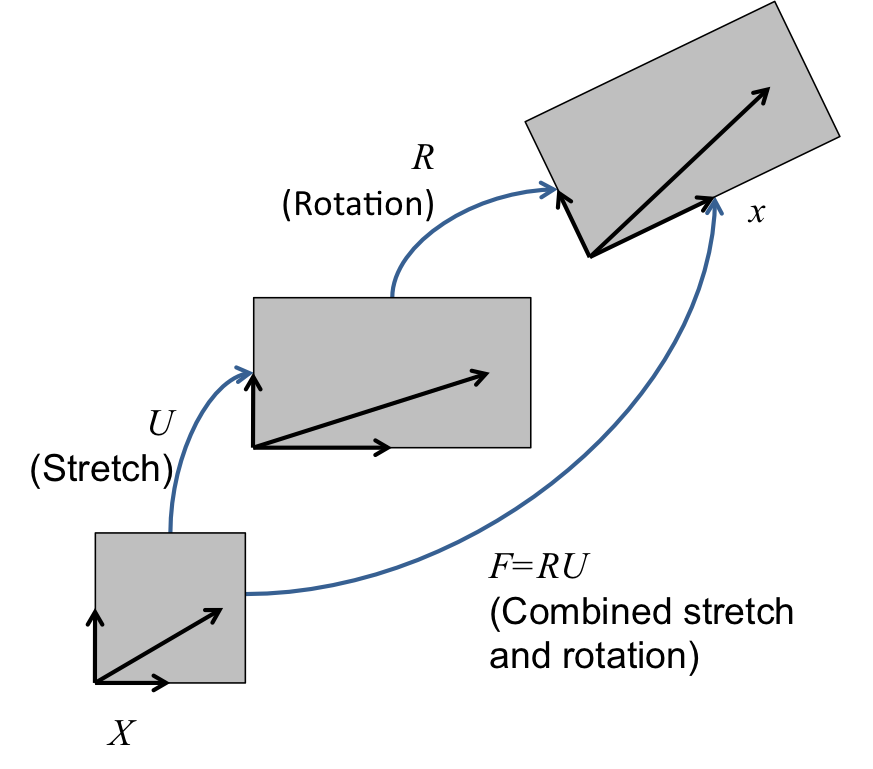
The deformation gradient can be viewed as the derivative of the current coordinates with respect to the original coordinates.
can be decomposed into pure rotation and pure stretch .
Mechanics: 3D
We begin with a complete set of data for step and seek the displacements and stresses at step . We first compute an incremental deformation gradient;
With , we next compute a strain increment that represents the rotation-free deformation from the configuration at to the configuration at . Following Rashid (1993), we seek the stretching rate :
Here, is the incremental stretch tensor, and is the incremental Green deformation tensor. Through a Taylor series expansion, this can be determined in a straightforward, efficient manner.
Mechanics: 3D (cont.)
is passed to the constitutive model as an input for computing at .
The next step is computing the incremental rotation, , where . Like for , an efficient algorithm exists for computing . It is also possible to compute these quantities using an eigenvalue/eigenvector routine.
With and , we rotate the stress to the current configuration.
Mechanics: Material Models
The material models for 1D, axisymmetric 2D, and 3D are formulated in an incremental fashion (think hypo-elastic).
Thus, the stress at the new step is the old stress plus a stress increment:
The incremental formulation is particularly useful for plasticity and creep models.
Let's add some more physics... Mechanics!
The following blocks have to be added or modified to our input file if we want to include mechanics behavior.
[Variables]
  [temperature]
  []
  [disp_x]
  []
  [disp_y]
  []
[]
[Physics]
  [SolidMechanics]
    [QuasiStatic]
      [block]
        block = 0
        add_variables = false
        strain = FINITE
        eigenstrain_names = thermal_eigenstrain
        temperature = temperature
      []
    []
  []
[]

[Kernels]
  [heat_conduction]
    type = HeatConduction
    variable = temperature
  []
  [heat_source]
    type = HeatSource
    variable = temperature
    value = 10000
  []
[]
[Materials]
  [heat_conductor]
    type = HeatConductionMaterial
    thermal_conductivity = 1
    block = 0
  []
  [elasticity_tensor1]
    type = ComputeIsotropicElasticityTensor
    block = 0
    youngs_modulus = 1e6
    poissons_ratio = 0.3
  []
  [thermal_expansion_strain1]
    type = ComputeThermalExpansionEigenstrain
    stress_free_temperature = 200
    thermal_expansion_coeff = 1.0e-4
    temperature = temperature
    eigenstrain_name = thermal_eigenstrain
    block = 0
  []
  [stress1]
    type = ComputeFiniteStrainElasticStress
    block = 0
  []
[]
Let's add some more physics... Mechanics!
The following blocks have to be added or modified to our input file if we want to include mechanics behavior.
[BCs]
  [leftright_temp]
    type = DirichletBC
    variable = temperature
    boundary = 'left right'
    value = 200
  []
  [leftright_disp_x]
    type = DirichletBC
    variable = disp_x
    boundary = 'left right'
    value = 0
  []
  [bottom_disp_y]
    type = DirichletBC
    variable = disp_y
    boundary = bottom
    value = 0
  []
[]
Heat Conduction + Mechanics: Results

Modules: Contact - Finite Element Contact Basics
A contact capability in a solid mechanics finite element code prevents the penetration of one domain into another, or part of one domain into itself.
Modules: Contact - Required Capabilities
A necessary but insufficient list:
Search
Exterior identification
Nearby nodes
Capture box
Binary search, e.g.
Contact existence
More geometric work
Penetration point
Enforcement
Formulation of contact force
Formulation of Jacobian
Interaction with other capabilities
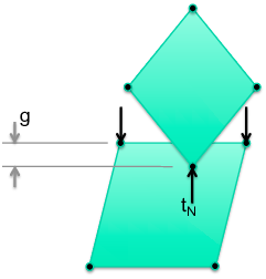
Contact: Overview
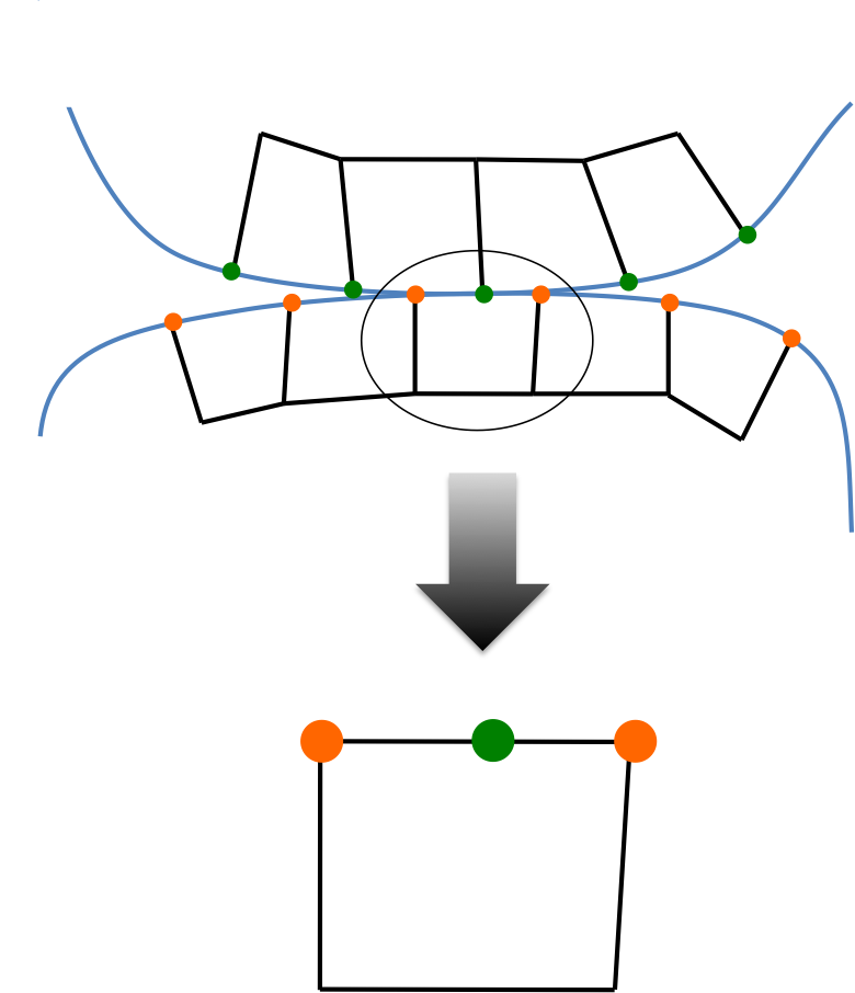
In node-face contact, nodes (green) may not penetrate faces (defined by orange nodes).
Forces must be determined to push against the two contacting bodies.
No force should be applied where the bodies are not in contact.
The contact forces must increase from zero as the bodies first come into contact.
Contact: Constraints
; the gap (penetration distance) must be non-positive
; the contact force must push bodies apart
; the contact force must be zero if the bodies are not in contact
; the contact force must be zero when constraints are formed and released
The gap in the normal direction for constraint is ( is the normal, denotes normal direction, is position of the secondary node, is position of the contact point, and is a matrix):
Contact: Contact Options
formulation: kinematicorpenaltyKinematic is more accurate but also harder to solve.
model:frictionless, glued, orcoulombFrictionless enforces the normal constraint and allows nodes to come out of contact if they are in tension. Glued ties nodes where they come into contact with no release. Coulomb is frictional contact with release.
friction_coefficientCoulomb friction coefficient.
penaltyThe penalty stiffness to be used in the constraint.
primaryThe surface corresponding to the faces in the constraint.
secondaryThe surface corresponding to the nodes in the constraint.
normal_smoothing_distanceDistance from face edge in parametric coordinates over which to smooth the normal. Helps with convergence. Try 0.1.
tension_releaseThe tension value that will allow nodes to be released. Defaults to zero.
Even more physics... CONTACT
The following blocks have to be added or modified to our input file if we want to include the effects of mechanical contact.
[Contact]
  [mechanical]
    model = frictionless
    formulation = mortar
    primary = bottom_square_top
    secondary = top_square_bottom
    c_normal = 1e+4
  []
[]
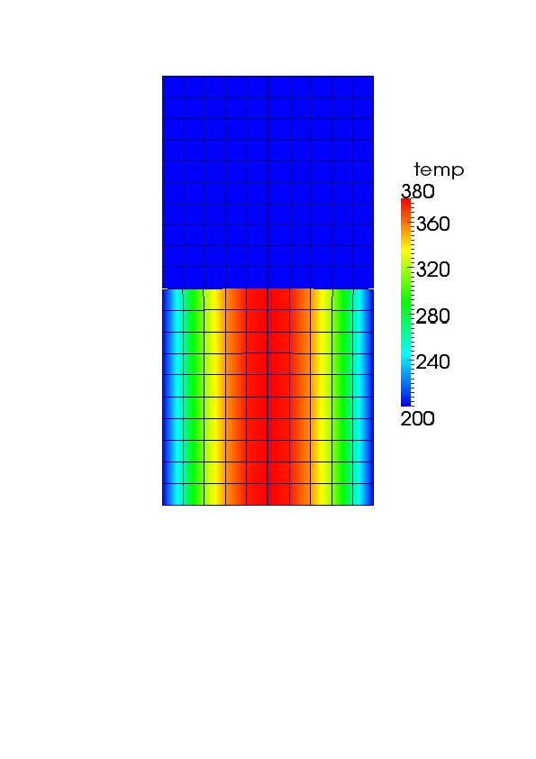
Heat Conduction + Mechanics + Contact: Results
q = 600
Bottom block heats and expands upward, but is not yet in contact
Blocks do not communicate thermally (no gap heat transfer)

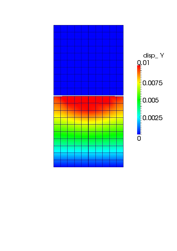
Heat Conduction + Mechanics + Contact: Results (cont.)
q = 600
Bottom block heats and expands upward, but is not yet in contact
Vertical displacement plots show curvature of top surface
Heat Conduction + Mechanics + Contact: Results (cont.)
q = 1500
Further heating and upward expansion brings blocks into contact; first at the center where the bottom block is hottest
Still, blocks do not communicate thermally (no gap heat transfer)
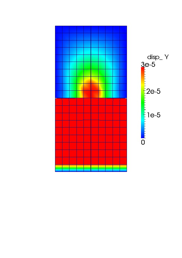
Heat Conduction + Mechanics + Contact: Results (cont.)
q = 1500
Contour scale is set to show displacement in top block resulting from mechanical contact
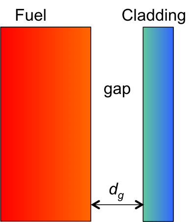
Modules: Heat Conduction: Gap Heat Transfer
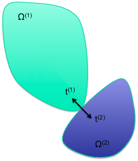
The principle is that the heat leaving one body must equal that entering another. For bodies and with heat transfer surface :
Gap heat transfer is modeled using the relation:
where is the total conductance across the gap, is the gas conductance, is the increased conductance due to solid-solid contact, and is the conductance due to radiant heat transfer.
In MOOSE modules, only the gas conductance is active by default.
The form of in MOOSE modules is:
where is the conductivity in the gap and is the gap distance.
Adding Thermal Contact
[MortarGapHeatTransfer]
  [thermal_contact]
    temperature = temperature
    boundary = bottom_square_top
    gap_conductivity = 1
    primary_boundary = bottom_square_top
    secondary_boundary = top_square_bottom
    primary_subdomain = mechanical_primary_subdomain
    secondary_subdomain = mechanical_secondary_subdomain
    gap_flux_options = 'CONDUCTION'
  []
[]
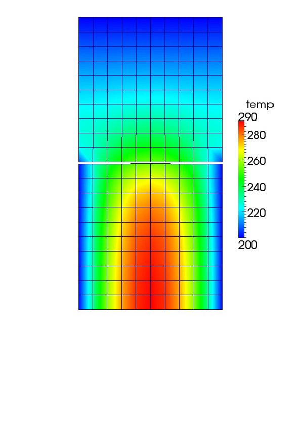
Heat Conduction + Mechanics + Contact + Thermal Contact: Results
q = 750
Heat tranfer occurs through the gap medium prior to mechanical contact
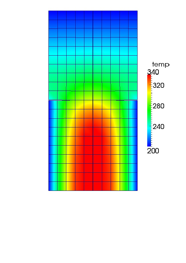
Heat Conduction + Mechanics + Contact + Thermal Contact: Results
q = 1330
Combined thermal and mechanical contact
General Modeling Advice
Advice
George Box:
... all models are approximations. Essentially, all models are wrong, but some are useful. However, the approximate nature of the model must always be borne in mind ...
Parsimony
Since all models are wrong the scientist cannot obtain a "correct" one by excessive elaboration. On the contrary following William of Occam he should seek an economical description of natural phenomena. Just as the ability to devise simple but evocative models is the signature of the great scientist so overelaboration and overparameterization is often the mark of mediocrity.
Advice
Worrying Selectively
Since all models are wrong the scientist must be alert to what is importantly wrong. It is inappropriate to be concerned about mice when there are tigers abroad.

Example Inputs
Let's go over some examples of input files:
Mechanics
Thermal
Contact
Most of the example inputs may be run with MOOSE modules and do not require BISON.
The examples will show some things to consider when modeling.
Mechanics Example
A Three-Point Bending Beam
Three-Point Bending Solution
Problem Statement
(depth into the plane)
Pa
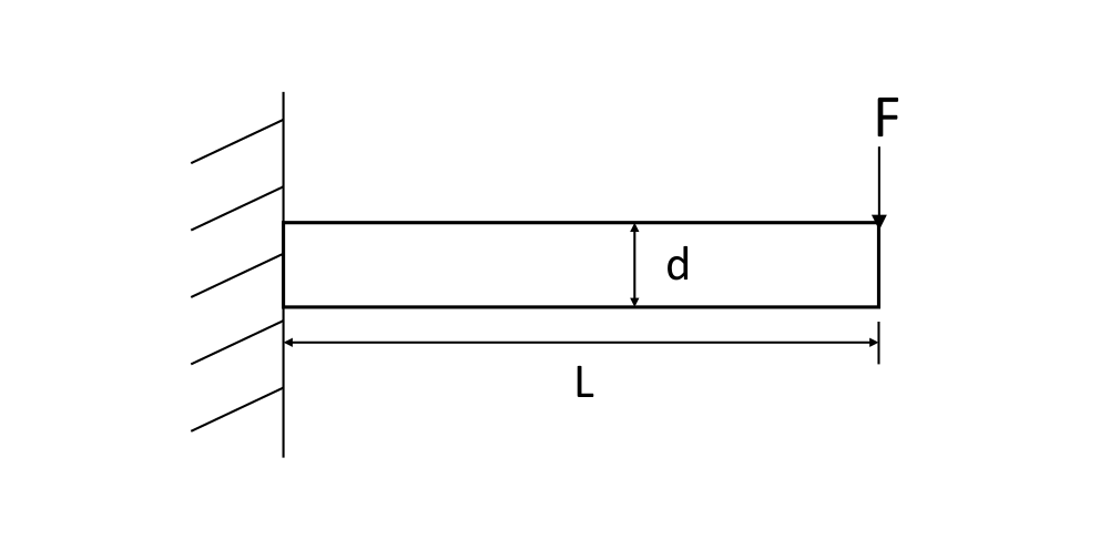
Solution
Tensor Mechanics Master Action
[Physics/SolidMechanics/QuasiStatic]
  [all]
    strain = FINITE
    add_variables = true
    generate_output = 'stress_xx stress_xy
                       stress_yy strain_xx
                       strain_xy strain_yy'
  []
[]
The primary or dependent variables in the PDEs (temperature, displacement) are defined in the
Variablesblock.A user-selected unique name is assigned for each variable.
An action can create and/or modify any number of the blocks in an input file. The Solid Mechanics physics creates several blocks, thus condensing the input file for a user.
Materials Block with Master Action
[Materials]
  [elasticity_tensor]
    type = ComputeIsotropicElasticityTensor
    youngs_modulus = 1e6
    poissons_ratio = 0.3
  []
  [stress]
    type = ComputeFiniteStrainElasticStress
  []
[]
Here, the elastic properties are specified by the
ComputeIsotropicElasticityTensorclass.Notice that the stress material property must be defined, while the strain is made by the solid mechanics physics and does not appear here.
Boundary Conditions
Need to prevent rigid body motion and load the beam.
[BCs]
  [free_end_moment]
    type = Pressure
    variable = disp_y
    component = 0
    boundary = right
    factor = 1
    function = loading_func
  []
  [FixedCenterLineX]
    type = DirichletBC
    variable = disp_x
    boundary = left
    value = 0.0
  []
  [FixedCenterLineY]
    type = DirichletBC
    variable = disp_y
    boundary = left
    value = 0.0
  []
  [FixedCenterLineZ]
    type = DirichletBC
    variable = disp_z
    boundary = left
    value = 0.0
  []
[]
Postprocessors
Shown here are a few postprocessors to help see how a simulation is running.
[Postprocessors]
  [num_lin_it]
    type = NumLinearIterations
  []
  [num_nonlin_it]
    type = NumNonlinearIterations
  []
  [tot_lin_it]
    type = CumulativeValuePostprocessor
    postprocessor = num_lin_it
  []
  [tot_nonlin_it]
    type = CumulativeValuePostprocessor
    postprocessor = num_nonlin_it
  []
  [alive_time]
    type = PerfGraphData
    section_name = Root
    data_type = TOTAL
  []
  [max_beam_deflection]
    type = NodalExtremeValue
    variable = disp_y
    boundary = 'right'
  []
[]
Mesh
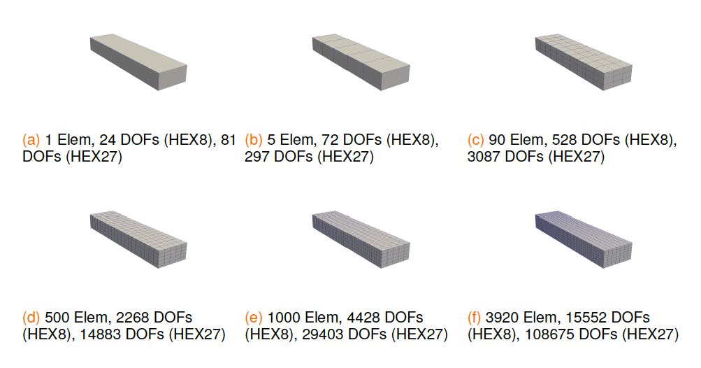
Results (Accuracy)
Elastic (HEX8 elements)
| Model | # Elem | # DOF | Max y-disp | Ratio to Exact | % Improve |
|---|---|---|---|---|---|
| 1x1x1 | 1 | 24 | -4.099E-3 | 0.040 | — |
| 5x1x1 | 5 | 72 | -6.981E-2 | 0.682 | 94.1 |
| 10x3x3 | 90 | 528 | -8.336E-2 | 0.814 | 16.3 |
| 20x5x5 | 500 | 2268 | -9.630E-2 | 0.940 | 13.4 |
| 40x5x5 | 1000 | 4428 | -1.008E-1 | 0.984 | 4.5 |
| 80x7x7 | 3920 | 15552 | -1.016E-1 | 0.992 | 0.8 |
Elastic (HEX27 elements)
| Model | # Elem | # DOF | Max y-disp | Ratio to Exact | % Improve |
|---|---|---|---|---|---|
| 1x1x1 | 1 | 81 | -7.763E-2 | 0.758 | — |
| 5x1x1 | 5 | 297 | -9.995E-2 | 0.976 | 22.3 |
| 10x3x3 | 90 | 3087 | -1.011E-1 | 0.987 | 1.1 |
| 20x5x5 | 500 | 14883 | -1.015E-1 | 0.991 | 0.4 |
Add Plasticity
What do you think?
More or less bend?
[Materials]
  [elasticity_tensor]
    type = ComputeIsotropicElasticityTensor
    youngs_modulus = 1e6
    poissons_ratio = 0.31
  []
  [stress]
    type = ComputeMultipleInelasticStress
    inelastic_models = 'isoplas'
  []
  [isoplas]
    type = IsotropicPlasticityStressUpdate
    yield_stress = 2.5e3
    hardening_constant = 1.85e5
  []
[]
Results (Accuracy)
Elastic-Plastic (HEX8 elements)
| Model | # Elem | # DOF | Max y-disp | % Improve |
|---|---|---|---|---|
| 1x1x1 | 1 | 24 | -4.131E-3 | — |
| 5x1x1 | 5 | 72 | -7.035E-2 | 94.1 |
| 10x3x3 | 90 | 528 | -9.039E-2 | 22.2 |
| 20x5x5 | 500 | 2268 | -1.212E-1 | 25.4 |
| 40x5x5 | 1000 | 4428 | -1.334E-1 | 9.1 |
| 80x7x7 | 3920 | 15552 | -1.377E-1 | 3.1 |
Elastic-Plastic (HEX27 elements)
| Model | # Elem | # DOF | Max y-disp | % Improve |
|---|---|---|---|---|
| 1x1x1 | 1 | 81 | -7.725E-2 | — |
| 5x1x1 | 5 | 297 | -1.396E-1 | 44.7 |
| 10x3x3 | 90 | 3087 | -1.349E-1 | 3.5 |
| 20x5x5 | 500 | 14883 | -1.381E-1 | 2.3 |
Add Creep
What do you think?
More or less bend?
[Materials]
  [elasticity_tensor]
    type = ComputeIsotropicElasticityTensor
    youngs_modulus = 1e6
    poissons_ratio = 0.31
  []
  [stress]
    type = ComputeMultipleInelasticStress
    inelastic_models = 'isoplas powerlawcrp'
  []
  [isoplas]
    type = IsotropicPlasticityStressUpdate
    yield_stress = 2.5e3
    hardening_constant = 1.85e5
  []
  [powerlawcrp]
    # Note that this model is load and time dependent
    type = PowerLawCreepStressUpdate
    #    coefficient = 3.125e-14
    #    n_exponent = 5.0
    coefficient = 5.0e-15
    n_exponent = 3.0
    m_exponent = 0.0
    activation_energy = 0.0
  []
  [thermal]
    type = HeatConductionMaterial
    specific_heat = 1.0
    thermal_conductivity = 100.
  []
  [density]
    type = StrainAdjustedDensity
    strain_free_density = 1.0
  []
[]
Results (Accuracy)
Elastic-Plastic with Creep (HEX8 elements)
| Model | # Elem | # DOF | Max y-disp | % Improve |
|---|---|---|---|---|
| 1x1x1 | 1 | 24 | -4.143E-3 | — |
| 5x1x1 | 5 | 72 | -7.390E-2 | 94.4 |
| 10x3x3 | 90 | 528 | -9.428E-2 | 21.6 |
| 20x5x5 | 500 | 2268 | -1.268E-1 | 25.6 |
| 40x5x5 | 1000 | 4428 | -1.398E-1 | 9.3 |
| 80x7x7 | 3920 | 15552 | -1.443E-1 | 3.1 |
Elastic-Plastic with Creep (HEX27 elements)
| Model | # Elem | # DOF | Max y-disp | % Improve |
|---|---|---|---|---|
| 1x1x1 | 1 | 81 | -7.977E-2 | — |
| 5x1x1 | 5 | 297 | -1.464E-1 | 45.5 |
| 10x3x3 | 90 | 3087 | -1.412E-1 | 3.7 |
| 20x5x5 | 500 | 14883 | -1.448E-1 | 2.5 |
Additional Comments
The analytical solution for the three-point bending problem assumes elastic material behavior.
The purpose of adding plasticity and creep was to demonstrate the affect of these material behaviors on the response of the beam to the same loading.
Thermal Example
Thermal Example Mesh
Square (on the left) and rectangle (on the right) are at different transient thermal conditions.
Structured 2D mesh that can either be made using CUBIT or MOOSE mesh generators.
Blocks and sidesets are defined to identify every boundary and surface.

Interpreting an Input File
[Variables]
  [T]
    initial_condition = 273.0
  []
[]

[Kernels]
  [heat]
    type = HeatConduction
    variable = T
  []
  [heat_ie]
    type = HeatConductionTimeDerivative
    variable = T
  []
  [heat_source_left]
    type = HeatSource
    block = 0 # left
    variable = T
    value = 100 # W/m2
  []
  [heat_sink_right]
    type = HeatSource
    block = 1 # right
    variable = T
    value = -15000 # W/m2
  []
[]
[BCs]
  # If not specified, defaults to Neumann = 0
  [left_top]
    type = DirichletBC
    boundary = top
    variable = T
    value = 293.0
  []
  [left_bottom]
    type = NeumannBC
    boundary = bottom
    variable = T
    value = -50.0 # W/m
  []
  [right_left]
    type = DirichletBC
    boundary = 7
    variable = T
    value = 400.0
  []
  [right_right]
    type = NeumannBC
    boundary = 5
    variable = T
    value = 100 # W/m
  []
[]
Interpreting an Input File
[Materials]
  [left_props]
    type = GenericConstantMaterial
    block = 0
    prop_names = 'density thermal_conductivity specific_heat'
    prop_values = '7850 4.45 4750'
  []
  [right_props]
    type = GenericConstantMaterial
    block = 1
    prop_names = 'density thermal_conductivity specific_heat'
    prop_values = '7850 10.5 4750'
  []
[]

[Executioner]
  type = Transient
  nl_rel_tol = 1e-6
  nl_abs_tol = 1e-9
  start_time = 0.0
  end_time = 360.0 #seconds
  dtmin = 0.1
  dtmax = 5.0

  [TimeStepper]
    type = ConstantDT
    dt = 2.0
  []
[]
[Postprocessors]
  [_dt]
    type = TimestepSize
    execute_on = 'initial timestep_end'
  []
  [avg_left]
    type = ElementAverageValue
    block = 0
    variable = T
    execute_on = 'initial timestep_end'
  []
  [avg_right]
    type = ElementAverageValue
    block = 1
    variable = T
    execute_on = 'initial timestep_end'
  []
  [max_left]
    type = ElementExtremeValue
    block = 0
    value_type = max
    variable = T
    execute_on = 'initial timestep_end'
  []
  [min_right]
    type = ElementExtremeValue
    block = 1
    value_type = min
    variable = T
    execute_on = 'initial timestep_end'
  []
  [avg_side_near_right]
    type = SideAverageValue
    boundary = right
    variable = T
    execute_on = 'initial timestep_end'
  []
Interpreting an Input File
  [avg_side_near_left]
    type = SideAverageValue
    boundary = 7
    variable = T
    execute_on = 'initial timestep_end'
  []
  [max_side_near_right]
    type = NodalExtremeValue
    boundary = right
    value_type = max
    variable = T
    execute_on = 'initial timestep_end'
  []
  [min_side_near_right]
    type = NodalExtremeValue
    boundary = 7
    value_type = min
    variable = T
    execute_on = 'initial timestep_end'
  []
  [peak_left]
    type = TimeExtremeValue
    postprocessor = max_left
    value_type = max
    execute_on = 'initial timestep_end'
  []
  [valley_right]
    type = TimeExtremeValue
    postprocessor = min_right
    value_type = min
    execute_on = 'initial timestep_end'
  []
[]
The documentation covers the MANY different postprocessors. We'll see that later.
Postprocessors have many roles, including providing data output, performance output, and needed input for other routines.
The parameter
execute_onis useful for specifying when postprocessors run.
Results
Change to Functions
[Functions]
  [left_heat]
    type = PiecewiseLinear
    x = '0 190 360'
    y = '25 100 0'
  []
  [left_left_flux]
    type = PiecewiseLinear
    x = '0 300 360'
    y = '-50 -50 0'
  []
  [right_cool]
    type = PiecewiseLinear
    x = '0 170 360'
    y = '25 0 -20000'
  []
  [right_left_T]
    type = PiecewiseLinear
    x = '0 360'
    y = '200 1000'
  []
[]
  [heat_source_left]
    type = HeatSource
    block = 0 # left
    variable = T
    function = left_heat
  []
  [heat_sink_right]
    type = HeatSource
    block = 1 # right
    variable = T
    function = right_cool
  []
[]
[BCs]
  # If not specified, defaults to Neumann = 0
  [left_top]
    type = DirichletBC
    boundary = top
    variable = T
    value = 293.0
  []
  [left_left]
    type = FunctionNeumannBC
    boundary = bottom
    variable = T
    function = left_left_flux
  []
  [right_left]
    type = FunctionDirichletBC
    boundary = 7
    variable = T
    function = right_left_T
  []
  [right_right]
    type = NeumannBC
    boundary = 5
    variable = T
    value = 100 # W/m
  []
[]
Function Results
Coolant Channel BC
An advanced convection boundary condition is set up in the
CoolantChannelsection.CoolantChannelroutine is actually a MOOSE "Action" setting up needed routines.Two working fluids are available: water and sodium.
Multiple correlation and subchannel geometries are available.
NOTE:
CoolantChannelwas designed for longer burnup simulations. Limited success has been had for fast transients.
[CoolantChannel]
  [convective_right_right]
    boundary = 5
    variable = T
    inlet_temperature = 600.0
    inlet_pressure = 455054.0
    inlet_massflux = 4520.72
    coolant_material = sodium
    flow_area = 2.22e-5
    hydraulic_diameter = 2.057e-3
    heated_perimeter = 1.835e-2
    heated_diameter = 4.84e-3
    number_axial_zone = 6
    htc_correlation_type = 3
    compute_enthalpy = true
  []
[]
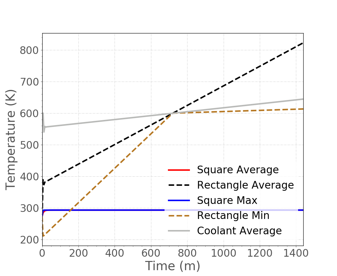
Coolant Channel BC Results
Notice the increased time scale for a larger time step size.
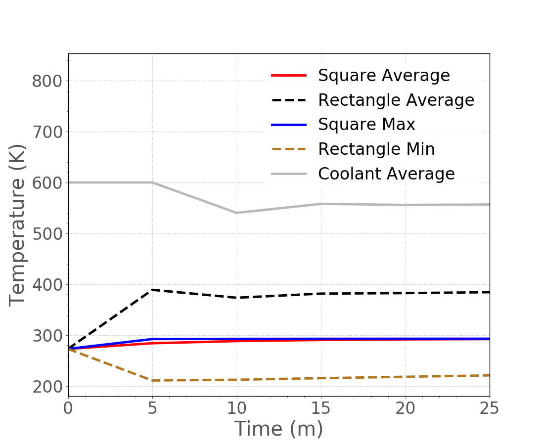
Coolant Channel BC Results Zoomed
Some instability at the beginning due to T calculation.
Gap Thermal Contact BC
Because gaps may close during a fuel performance simulation, these gaps are not meshed.
ThermalContactsection handles heat transfer across an un-meshed gap.ThermalContactroutine is actually a MOOSE "Action" setting up needed routines.Does not require mechanics to be included in the simulation.
Basic capability for mass transport across a gap.
The "primary" boundary usually has larger elements than the "secondary" boundary.
This follows the mechanical contact convention for sideset assignment.
[ThermalContact]
  [connect_T]
    type = GapHeatTransfer
    variable = T
    primary = 7
    secondary = right
    quadrature = true
    gap_conductivity = 1.0
    min_gap = 1e-3
  []
[]
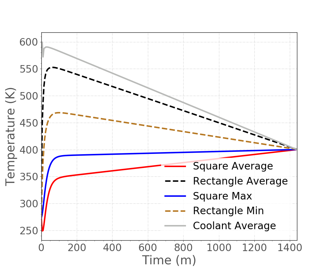
Gap Thermal Contact BC Results
Transient Considerations: Coolant
If CoolantChannel is not working for a transient simulation, other convection boundary conditions may help.
[BCs]
  [convective_clad_surface]
    type = ConvectiveFluxFunction
    boundary = 2
    variable = temperature
    coefficient = 1.0 # multiplies HTC
    T_infinity = Tinf_fun
    coefficient_function = htc_fun
  []
[]
[Functions]
  [htc_fun]
    type = PiecewiseBilinear
    axis = 1 # y
    data_file = 'scaled_htc.csv'
  []
  [Tinf_fun]
    type = PiecewiseBilinear
    axis = 1 # y
    data_file = 'scaled_Tinf.csv'
  []
[]
ConvectiveFluxFunction may use functions to provide convection coefficient and T values.
[BCs]
  [right]
    type = CoupledConvectiveHeatFluxBC
    variable = u
    boundary = right
    alpha = 'alpha_liquid alpha_vapor'
    htc = 'Hw_liquid Hw_vapor'
    T_infinity = 'T_infinity_liquid T_infinity_vapor'
  []
[]
[AuxVariables]
  [T_infinity_liquid]
  []
  [Hw_liquid]
  []
  [alpha_liquid]
  []
  [T_infinity_vapor]
  []
  [Hw_vapor]
  []
  [alpha_vapor]
  []
[]
CoupledConvectiveHeatFluxBC may approximate two-phase coolant. The AuxVariables for input may be set by coupled applications or AuxKernels.
Transient Considerations: Numerical Artifacts
Numerical artifacts producing non-physical results may occur for transients, creating thermal "shock-like" heat transfer.
For example, using the thermal mesh from before, square's heat generation is extremely large and fast.
Rectangle has a right-side Dirichlet boundary held at 293 K.
Thermal contact exists between square and rectangle.
Square and rectangle both start at 273 K and are the same material.
The heat generation in square decreases substantially after 0.1 sec.
Time step size is a constant 0.01 sec.
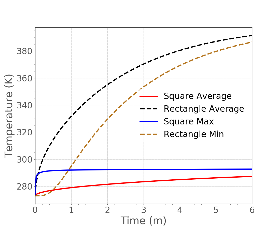
Artifact Results
Something's Not Right
TimeExtremeValue and ElementExtremeValue postprocessors of a "min" type show non-physical cooling occurring in the cladding.
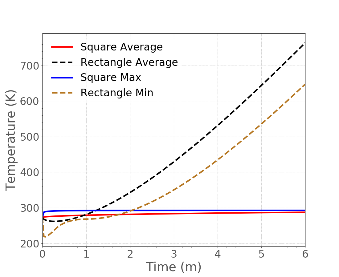
Artifact Fix
Sort of feels like artificial diffusion; let's see what more elements do.
Contact Example
Contact Problem

2D plane geometry
Two blocks
Fixed at bottom and left sides of lower block
Displacement BC at top of upper block in vertical direction
Contact Block
[Contact]
  [interface]
    secondary = 4
    primary = 2
    model = frictionless
    formulation = penalty
    penalty = 1e+3
  []
[]
primaryThe surface corresponding to the faces in the constraint.
secondaryThe surface corresponding to the nodes in the constraint.
Contact Block (Cont.)
[Contact]
  [interface]
    secondary = 4
    primary = 2
    model = frictionless
    formulation = penalty
    penalty = 1e+3
  []
[]
formulation: kinematicorpenalty- Kinematic is more accurate but also harder to solve.
model: frictionless, glued,orcoulomb- Frictionless enforces the normal constraint and allows nodes to come out of contact if they are in tension.
- Glued ties nodes where they come into contact, with no release.
- Coulomb is frictional contact with release.
penalty- The penalty stiffness to be used in the constraint.
Contact Solution - Penalty Approach

Penalty = 1e3 (i.e., spring force between contact surfaces)
Obvious overlap of bodies (un-physical solution!)
Contact Solution - Higher Penalty

Penalty = 1e9
No obvious overlap of bodies (more realistic solution)
Contact Solution - Solution Comparison

Penetration decreases with increasing penalty value.
Kinematic Formulation
Frictionless Contact
[Contact]
  [interface]
    secondary = 4
    primary = 2
    model = frictionless
    formulation = kinematic
  []
[]
Glued Contact
[Contact]
  [interface]
    secondary = 4
    primary = 2
    model = glued
    formulation = kinematic
  []
[]
Note that no penalty value is necessary.
Contact Solution - Comparing Contacts
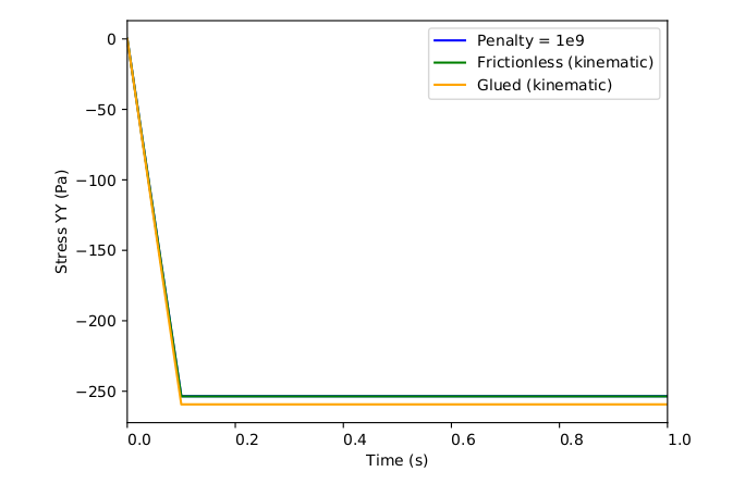
Stress YY similar for different formulations
Glued formulation slightly higher due to constraint on tangential node
Visualizing Results
Output Files
Preferred output for MOOSE applications is ExodusII (Schoof and Yarberry, 1996) binary format. Several options exist for visualizing ExodusII files:
ParaView
Open-source general visualization tool
Ensight
Commercial general visualization tool
Peacock
MOOSE GUI has integrated postprocessor
Live update of results while model is running
Blot
Command-line visualization tool
Part of SEACAS suite of codes for working with Exodus files
Easily scripted, useful for generating x-y plots
Patran
Commercial pre- and post-processor, requires Exodus plugin
VisIt
Open-source general visualization tool
ParaView
Open-source GUI-based visualization tool
Provides readers for many data formats, including Exodus
Intended for visualization of very large datasets
- Remote parallel rendering
- Some behavior of the user interface driven by that emphasis.
- Strong preference toward loading minimal data into memory.
Thin GUI layer on top of VTK open-source visualization toolkit (Kitware).
- Same software used for displaying graphics in Cubit
Brief usage tutorial provided in the following slides

Setting an Alias
To allow opening of ExodusII files from the command line, adding an alias can be useful.
Open your
.bash_profileon Mac or.bashrcon Linux and add an alias to the ParaView executable. For example, for ParaView version 5.6.0 on a Mac:
alias paraview="/Applications/ParaView-5.6.0.app/Contents/MacOS/paraview"
This allows you to open a specific ExodusII file via:
paraview my_awesome_file.e
Brief ParaView Tutorial
We will use a BISON example problem to demonstrate functionality within ParaView.
Additional tutorials for ParaView can be found here.
Other Postprocessing Options
BISON can output global scalar quantities of interest to a CSV file for further post-processing using Postprocessors.
The CSV can be imported into Excel.
The CSV can be read into Python for journal quality plots through matplotlib.
BISON can also output global scalar quantities of interest along a specified line or boundary using VectorPostprocessors.
Mesh Generation
BISON Input Files
BISON requires two files in order to run.
The first of these is an input text file.
The second is an input mesh file.
The default format is ExodusII (Schoof and Yarberry, 1996).
The creation of the mesh file is the subject of this section.
Meshes can be created external to the input text file.
Meshes can be created internal to the input text file.
Creating Mesh Input Files
CUBIT from Sandia National Laboratories (Sandia National Laboratories, 2008).
Use CUBIT directly.
Use scripts to drive CUBIT.
Create an Abaqus file and import that into BISON instead.
Output ExodusII from Patran or Ansys.
CUBIT can be licensed from Sandia (free for government use). A commercial version, Trelis, is available from csimsoft.
CUBIT Interface
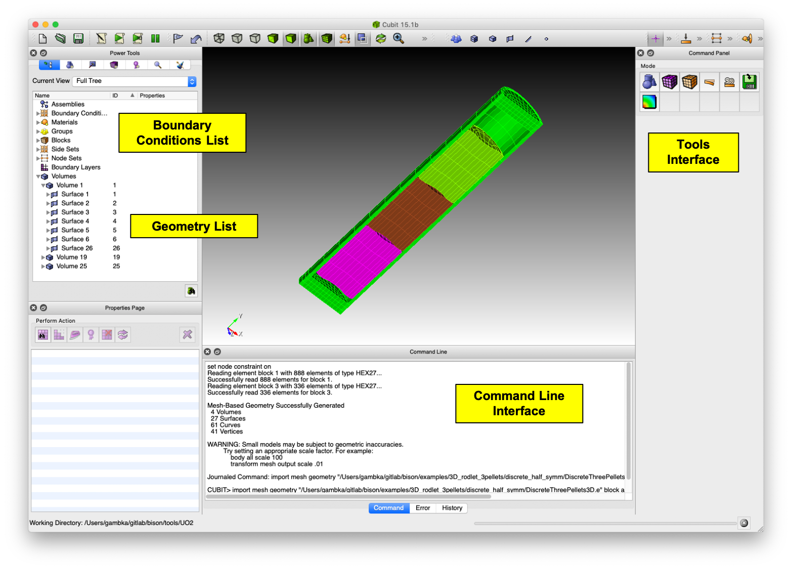
CUBIT Capabilities
Generating a solid model
Importing a solid model
Automatically generating a mesh for simple geometries
Creating 1D, 2D, or 3D meshes
Assigning blocks, side sets, and node sets
Being driven by a GUI, command line, journal file, or Python
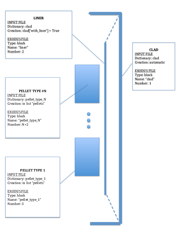
BISON's Mesh Generation Scripts
Shell and Python scripts for mostly automatic fuel rod mesh generation are in
bison/tools/UO2.Relevant files are:
mesh_script.sh: Sets up environment variables. Callsmesh_script.pyandmesh_script_input.py.mesh_script.py: Main script. Interfaces with CUBIT. Handles both 2D and 3D geometries. User should not have to modify this file.mesh_script_input.pyInput file. Defines geometry and mesh parameters using Python dictionaries.
Mesh input file review: Fuel
In the following slides, we will go over the options available in the mesh_script_input.py file.
#/*************************************************/
#/*           DO NOT MODIFY THIS HEADER           */
#/*                                               */
#/*                     BISON                     */
#/*                                               */
#/*    (c) 2015 Battelle Energy Alliance, LLC     */
#/*            ALL RIGHTS RESERVED                */
#/*                                               */
#/*   Prepared by Battelle Energy Alliance, LLC   */
#/*     Under Contract No. DE-AC07-05ID14517      */
#/*     With the U. S. Department of Energy       */
#/*                                               */
#/*     See COPYRIGHT for full restrictions       */
#/*************************************************/

#!/usr/bin/env python2.5

""" Pellet default geometry
Pellet1['outer_radius'] = 0.0041
Pellet1['inner_radius'] = 0
Pellet1['height'] = 2*5.93e-3
Pellet1['dish_spherical_radius'] = 1.01542e-2
Pellet1['dish_depth'] = 3e-4
Pellet1['chamfer_width'] = 5.0e-4
Pellet1['chamfer_height'] = 1.6e-4
#/*************************************************/
#/*           DO NOT MODIFY THIS HEADER           */
#/*                                               */
#/*                     BISON                     */
#/*                                               */
#/*    (c) 2015 Battelle Energy Alliance, LLC     */
#/*            ALL RIGHTS RESERVED                */
#/*                                               */
#/*   Prepared by Battelle Energy Alliance, LLC   */
#/*     Under Contract No. DE-AC07-05ID14517      */
#/*     With the U. S. Department of Energy       */
#/*                                               */
#/*     See COPYRIGHT for full restrictions       */
#/*************************************************/

#!/usr/bin/env python2.5

""" Pellet default geometry
Pellet1['outer_radius'] = 0.0041
Pellet1['inner_radius'] = 0
Pellet1['height'] = 2*5.93e-3
Pellet1['dish_spherical_radius'] = 1.01542e-2
Pellet1['dish_depth'] = 3e-4
Pellet1['chamfer_width'] = 5.0e-4
Pellet1['chamfer_height'] = 1.6e-4
"""

# Pellet Type 1
# Obligatory parameters
Pellet1= {}
Pellet1['type'] = 'discrete'
Pellet1['quantity'] = 10
Pellet1['mesh_density'] = 'coarse'

Pellet1['outer_radius'] = 0.0041
Pellet1['inner_radius'] = 0
Pellet1['height'] = 2*5.93e-3
Pellet1['dish_spherical_radius'] = 1.01542e-2
Pellet1['dish_depth'] = 3e-4
Pellet1['chamfer_width'] = 5.0e-4
Pellet1['chamfer_height'] = 1.6e-4

# Obligatory parameters
Pellet2= {}
Pellet2['type'] = 'discrete'
Pellet2['quantity'] = 1
Pellet2['mesh_density'] = 'coarse'

Pellet2['outer_radius'] = 0.00278
Pellet2['inner_radius'] = 0.0009
Pellet2['height'] = 2*0.106
Pellet2['dish_spherical_radius'] = 0
Pellet2['dish_depth'] = 0
Pellet2['chamfer_width'] = 0
Pellet2['chamfer_height'] = 0
Mesh input file review: Pellet stack
# Pellet Collection

pellets = [Pellet1]
#pellets = [Pellet1, Pellet2, Pellet1]

# Stack options
pellet_stack = {}
pellet_stack['default_parameters'] = False

pellet_stack['interface_merge'] = 'all'   # choose between 'point', 'none' or 'all'
pellet_stack['higher_order'] = False
pellet_stack['angle'] = 0
default_parametersuse default parameters without considering below parametersinterface_mergepoint(default) common vertex (2D) or curve (3D)nonenot merged
higher_orderFalse: QUAD4 (2D) or HEX8 (3D).True: QUAD8 (2D) or HEX27 (3D).
angle0: create a 2D-RZ geometry.
0: create a 3D stack of the specified angle ()
Mesh input file review: Clad
Defines clad geometric parameters. Please note:
mesh_density: clad mesh depends on fuel mesh.clad_width: this parameter is the total width of the clad, including the liner.
# Clad: Geometry of the clad
clad = {}
clad['mesh_density'] = 'coarse'
clad['gap_width'] = 8e-5
clad['bot_gap_height'] = 1e-3
clad['clad_thickness'] = 5.6e-4
clad['top_bot_clad_height'] = 2.24e-3
clad['plenum_fuel_ratio'] = 0.045

clad['with_liner'] = False
clad['liner_width'] = 5.0e-5
Mesh input file review: Meshing parameters
Mesh parameters are also stored in a dictionary.
The name of the dictionary must be the same as defined in the pellet type block (
mesh_density).
# Meshing parameters
mesh = {}
mesh['default_parameters'] = False

# Parameters of mesh density 'coarse'
coarse = {}
coarse['pellet_r_interval'] = 6
coarse['pellet_z_interval'] = 2
coarse['pellet_dish_interval'] = 3
coarse['pellet_flat_top_interval'] = 2
coarse['pellet_chamfer_interval'] = 1
coarse['clad_radial_interval'] = 3
coarse['clad_sleeve_scale_factor'] = 1
coarse['cap_radial_interval'] = 6
coarse['cap_vertical_interval'] = 3
coarse['pellet_slices_interval'] = 4
coarse['pellet_angular_interval'] = 6
coarse['clad_angular_interval'] = 12

# Parameters of the mesh density 'medium'
medium = {}
medium['pellet_r_interval'] = 11
medium['pellet_z_interval'] = 3
medium['pellet_dish_interval'] = 6
medium['pellet_flat_top_interval'] = 3
medium['pellet_chamfer_interval'] = 2
medium['clad_radial_interval'] = 4
medium['clad_sleeve_scale_factor'] = 1
medium['cap_radial_interval'] = 4
medium['cap_vertical_interval'] = 3
medium['pellet_slices_interval'] = 16
medium['pellet_angular_interval'] = 12
medium['clad_angular_interval'] = 16
For a smeared pellet, the mesh density of the fuel is controlled by the parameters
pellet_r_intervalandpellet_z_interval. Otherpellet*parameters are used with a discrete geometry.clad_sleeve_scale_factor1: same vertical density as the fuel
: higher density
: smaller density
Recommend that
Output review: Boundary conditions
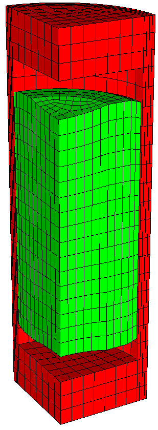
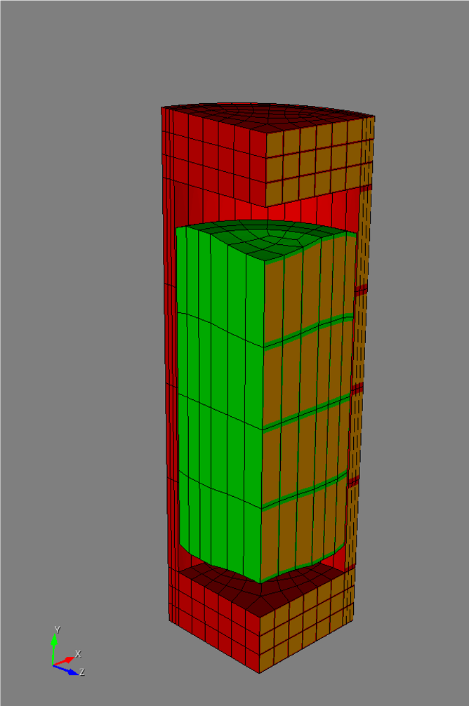
3D Boundary Conditions (180-degree model)
3D Mesh
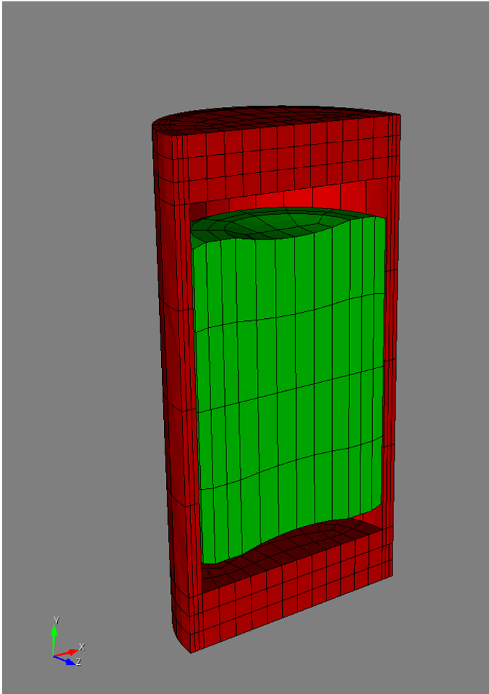
Sideset 99 Definition
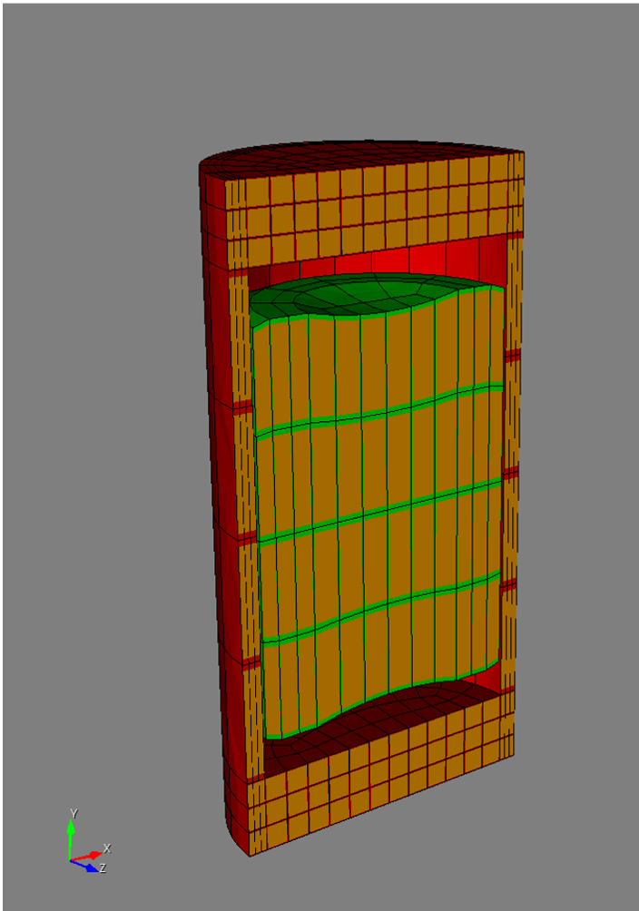
3D Boundary Conditions (90-degree model)
3D Mesh
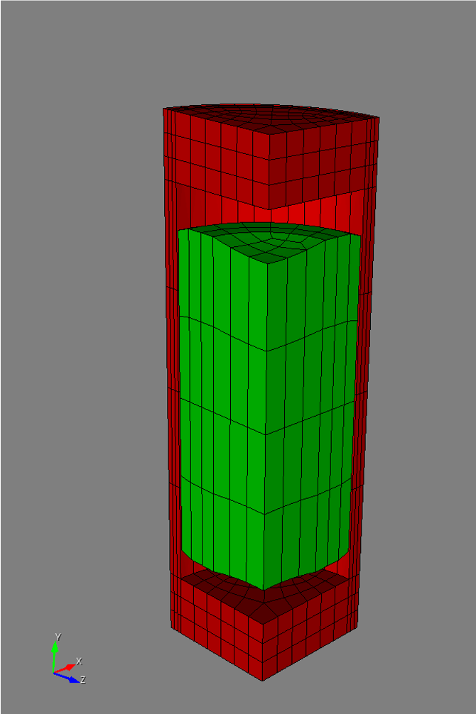
Sideset 98 Definition
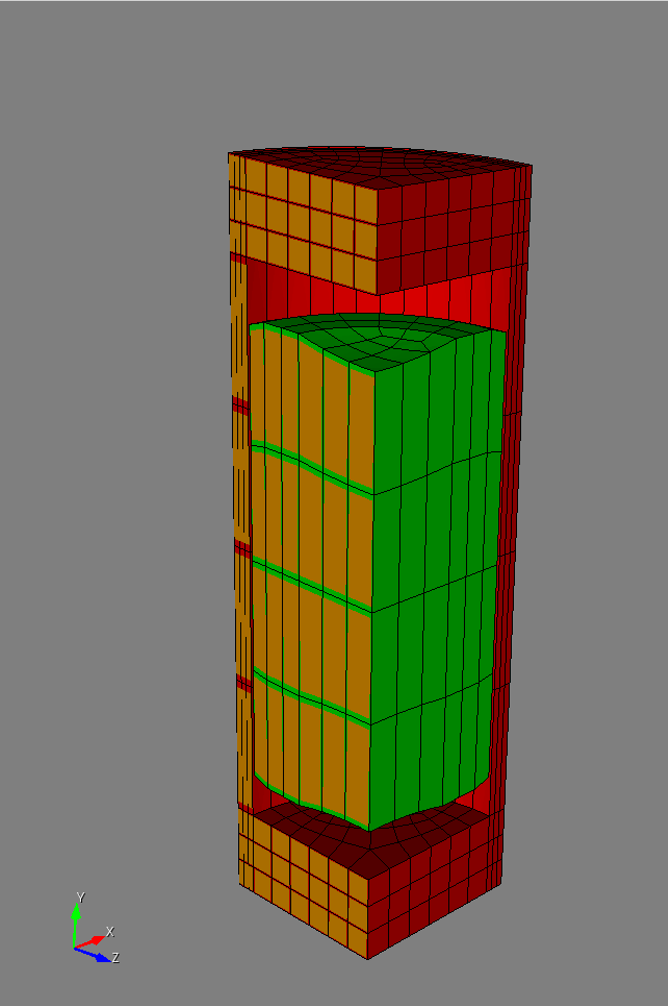
Sideset 99 Definition
Mesh script: Wrap-up
Geometry and mesh parameters are defined in the input file for 2D or 3D geometry
No interaction with the main script is required
In the Exodus file, blocks have these names:
clad,liner, andpellet_type_#
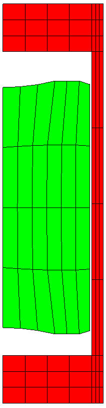
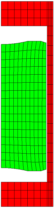
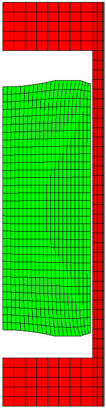
Mesh Examples
Coarse
Medium
Fine
3D Medium
Mesh Generators
MOOSE and BISON also have internal meshing capabilities. Capabilities specific to BISON include:
A complete list of all available MeshGenerators can be found here.
SmearedPelletMeshGenerator
Used to create 2D-RZ axisymmetric smeared pellet meshes.
[Mesh]
  [gen]
    type = FuelPinMeshGenerator
    clad_top_gap_height = 6.0413e-4
    coating_thickness = 1e-4
    nx_coating = 2
    clad_mesh_density = customize
  []
[]
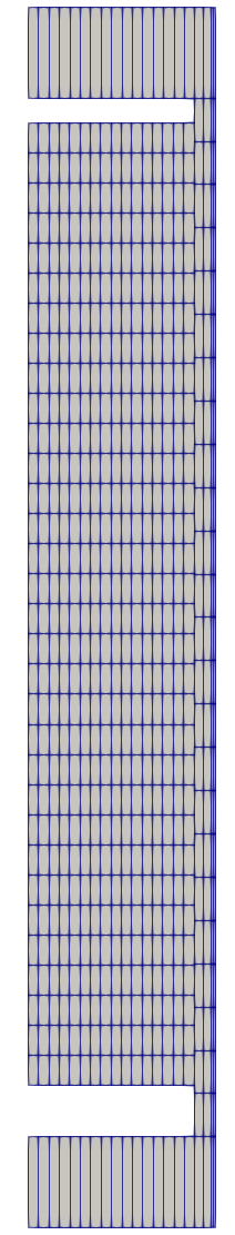
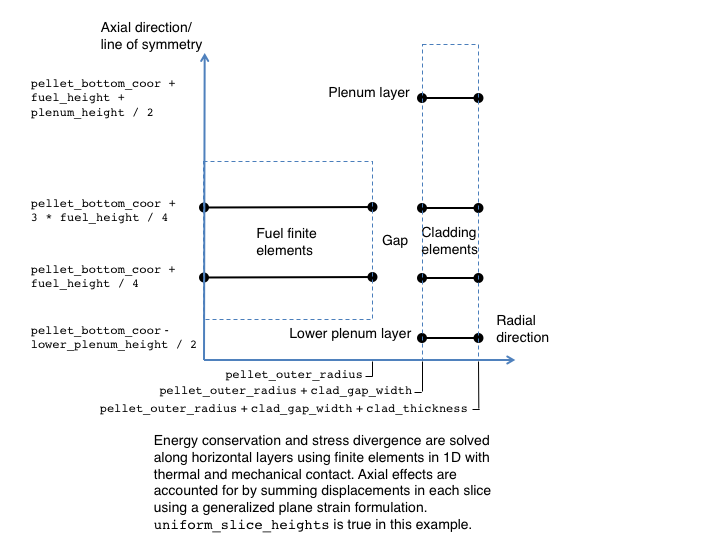
Layered1DMeshGenerator
Used to create 2D-RZ axisymmetric layered 1D meshes.
[Mesh]
  coord_type = RZ
  [layered1D_mesh]
    type = Layered1DMeshGenerator
    slices_per_block = 30
    pellet_outer_radius = 4.565e-3
    clad_gap_width = 0.085e-3
    clad_thickness = 0.725e-3
    fuel_height = 0.480
    plenum_height = 0.262416
    pellet_mesh_density = customize
    clad_mesh_density = customize
    nx_p = 11
    nx_c = 5
  []
  patch_update_strategy = auto
  partitioner = centroid
  centroid_partitioner_direction = y
[]
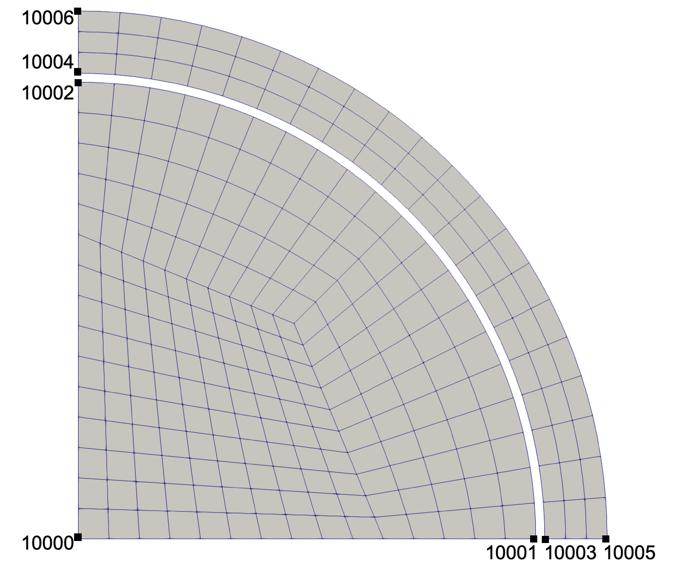
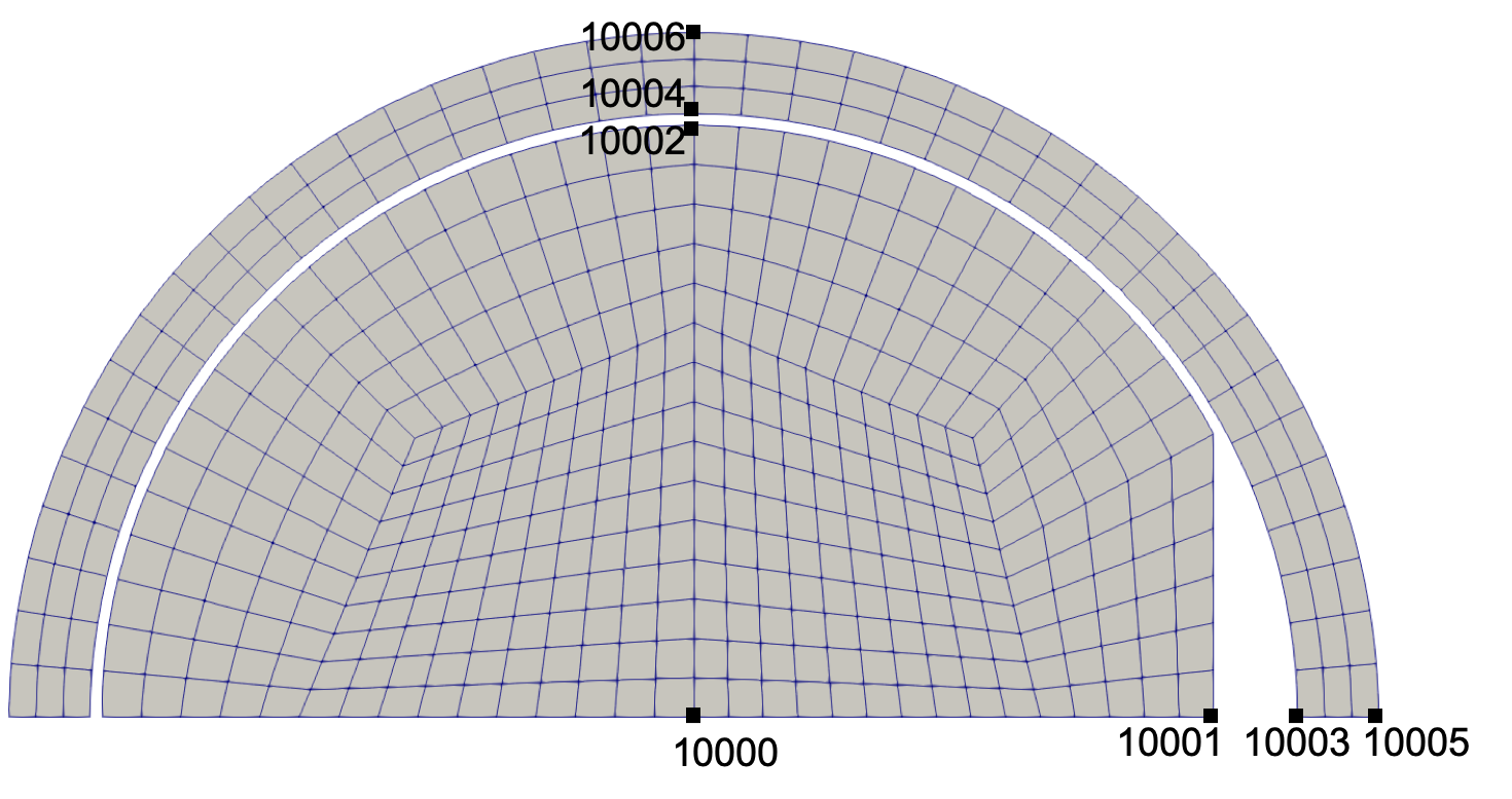
CircularCrossSectionMeshGenerator
Used to create 2D plane strain meshes.
[Mesh]
  [ccsmg]
    type = CircularCrossSectionMeshGenerator
    num_sectors = 20
    elements_per_ring = '5 0 3'
    block_names = 'fuel null clad'
    coordinates = '0.0041 0.00418 0.00474'
  []
[]
MPSCircularCrossSectionMeshGenerator
Used to create 2D plane strain meshes containing an MPS.
[Mesh]
  [mpsccsmg]
    type = MPSCircularCrossSectionMeshGenerator
    num_sectors = 20
    elements_per_ring = '5 0 3'
    block_names = 'fuel null clad'
    coordinates = '0.0041 0.00418 0.00474'
    mps_depth = 0.0005
  []
[]
Layered2DMeshGenerator
Used to create 2D plane strain layered 2D meshes.
[Mesh]
  [l2Dmg]
    type = Layered2DMeshGenerator
    num_sectors = 10
    slices_per_block = '2'
    pellet_bottom_coor = 0.0
    pellet_mesh_density = coarse
    clad_mesh_density = coarse
    include_plenum = false
    fuel_height = 10e-3
    additional_block_names = 'null capsule'
    additional_elements_per_ring = '0 1'
    additional_ring_thicknesses = '100e-6 500e-6'
  []
[]
PlateMeshGenerator
Creates a 3D mesh of a nuclear fuel plate, including fuel, liner, and cladding.
[Mesh]
  [plate]
    type = PlateMeshGenerator
    fuel_dimensions = '.5 .5 .05'
    liner_thickness = .05
    cladding_thicknesses = '0.5 1 0.25 0.25 0.05 0.1'
    number_fuel_elements = '8 2 1'
    number_cladding_elements = '2 2 2 2 2 3'
    number_liner_elements = 3
    radius = 2
    move_directions = 'z'
    move_functions = '0.2*(x+1)*(y+0.5)/2.0*z'
  []
[]
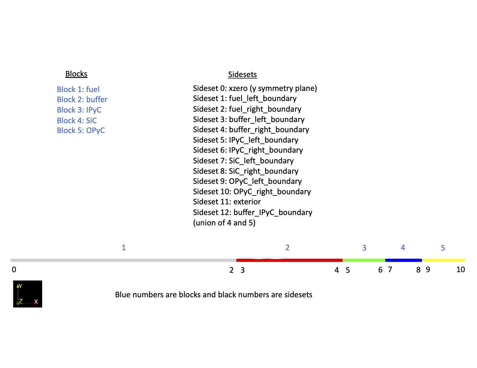
TRISO1DMeshGenerator
Creates a 1D mesh of a TRISO fuel particle by specifying the radial coordinates corresponding to the interface between different materials within the particle.
[Mesh]
  coord_type = RSPHERICAL
  [gen]
    type = TRISO1DMeshGenerator
    elem_type = EDGE3
    coordinates = '0 2.485e-4 3.425e-4 3.425e-4 3.835e-4 4.195e-4 4.595e-4'
    mesh_density = '6 6 0 6 8 6'
    block_names = 'fuel buffer IPyC SiC OPyC'
  []
[]
TRISO1DFiveLayerMeshGenerator
Creates a 1D mesh of a TRISO fuel particle by specifying the radius of the fuel kernel and the thicknesses of the buffer, IPyC, SiC, and OPyC layers. This mesh generator is primarily used for failure analyses.
[Mesh]
  coord_type = RSPHERICAL
  [gen]
    type = TRISO1DFiveLayerMeshGenerator
    elem_type = EDGE3
    kernel_radius = 2.485e-4
    buffer_thickness = 9.4e-5
    IPyC_thickness = 4.1e-5
    SiC_thickness = 3.6e-5
    OPyC_thickness = 4.0e-5
    kernel_mesh_density = 6
    buffer_mesh_density = 6
    IPyC_mesh_density = 6
    SiC_mesh_density = 8
    OPyC_mesh_density = 6
  []
[]
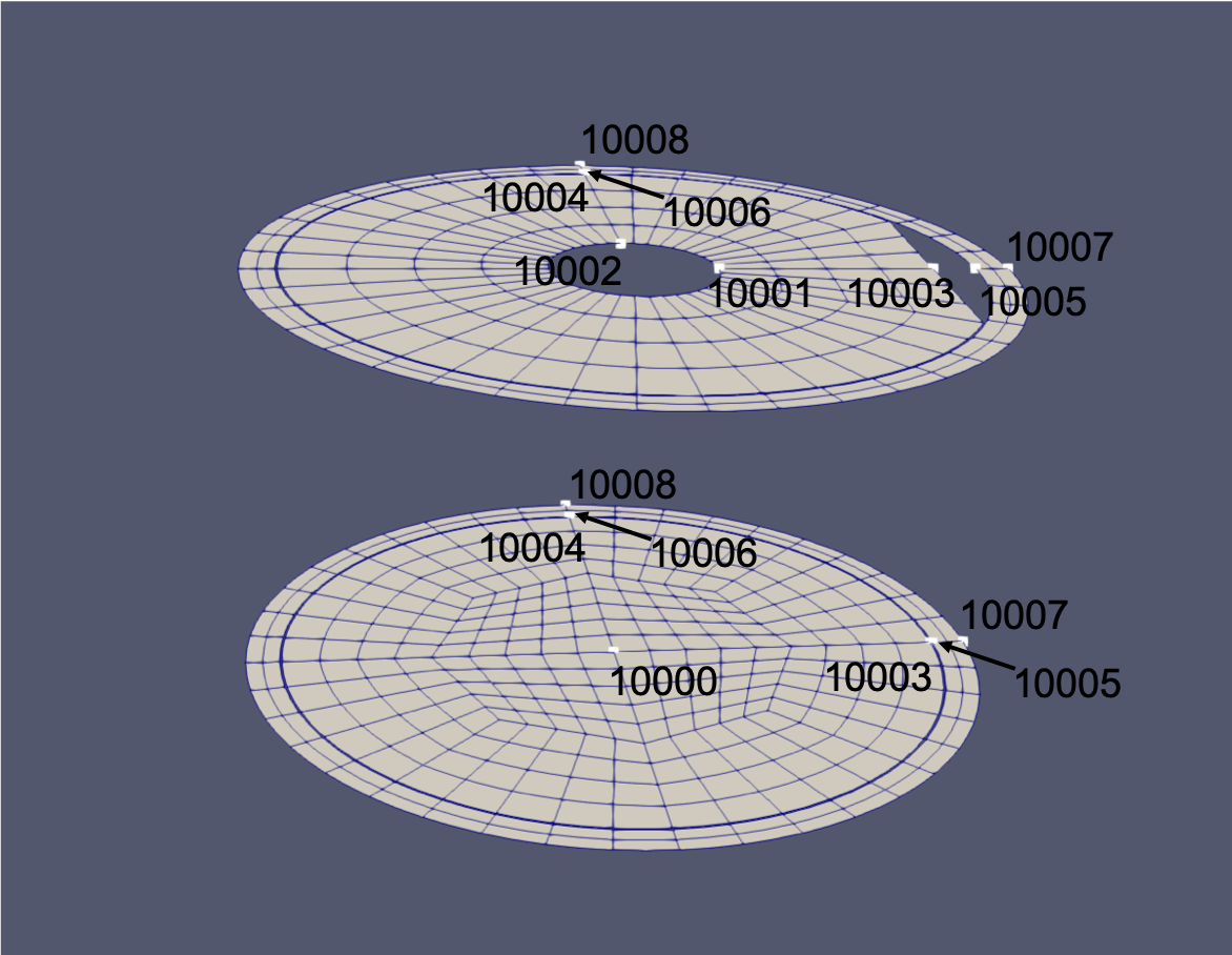
TRISO2DMeshGenerator
Creates a 2D mesh of a TRISO fuel particle.
[Mesh]
  coord_type = RZ
  [mesh]
    type = TRISO2DMeshGenerator
    elem_type = quad4
    coordinates = '0 2.485e-4 3.425e-4 3.425e-4 3.835e-4 4.195e-4 4.595e-4'
    mesh_density = '6 6 0 6 8 6'
    block_names = 'fuel buffer IPyC SiC OPyC'
    num_sectors = 20
  []
[]
LWR Capabilities
BISON LWR Capabilities
General Capabilities
3D, 2D-RZ, 1D fully coupled thermo-mechanics
Large deformations
Parallel
Meso-scale informed
Oxide Fuel Behavior
Temperature/burnup/porosity dependent material properties
Volumetric heat generation
Thermal and fission product swelling, and densification strains
Thermal and irradiation creep
Fuel fracture via relocation and smeared cracking
Fission gas release (2 stages)
transient release
grain growth/sweeping
athermal release
Temperature
Gap/Plenum Behavior
Gap heat transfer with
Mechanical contact
Plenum pressure as a function of:
evolving gas volume (from mechanics)
gas mixture (FGR)
gas temperature approximation
Cladding Behavior
Thermal and irradiation creep
Thermal expansion
Irradiation growth
Plasticity
Hydride damage
Coolant Channel
Closed channel thermal hydraulics with heat transfer coefficients
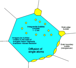
Fission Gas Behavior
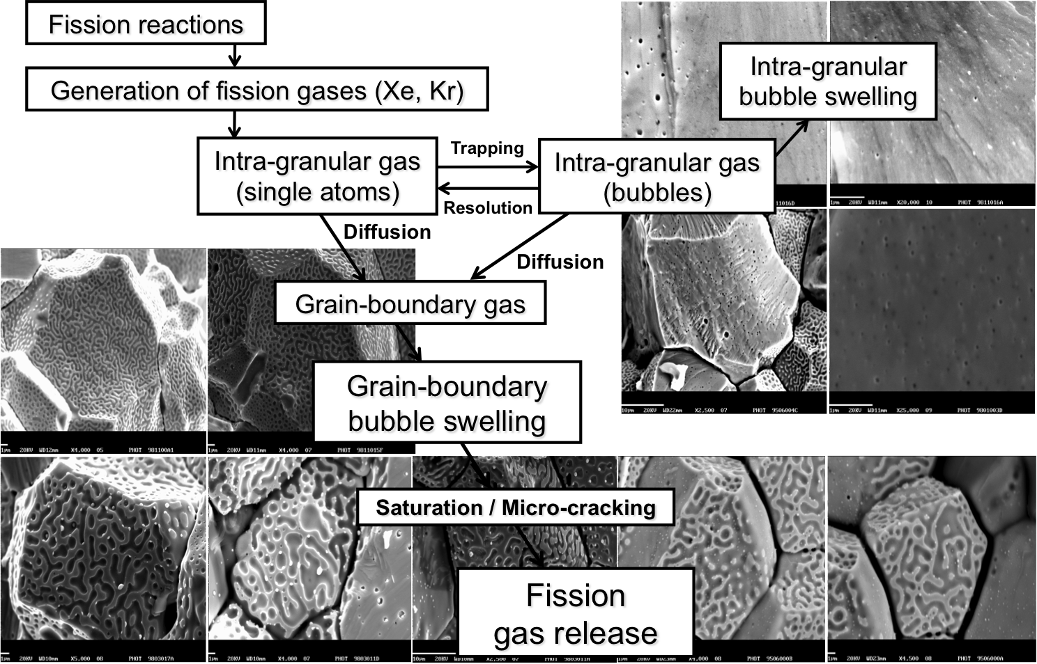
BISON Fission Gas Model
Physics-based model that describes the different stages of fission gas behavior
Gas generation
Intra-granular diffusion to grain boundaries
Bubble development at grain boundaries and associated fuel swelling
Fission gas release due to grain boundary saturation
Fission gas release due to micro-cracking
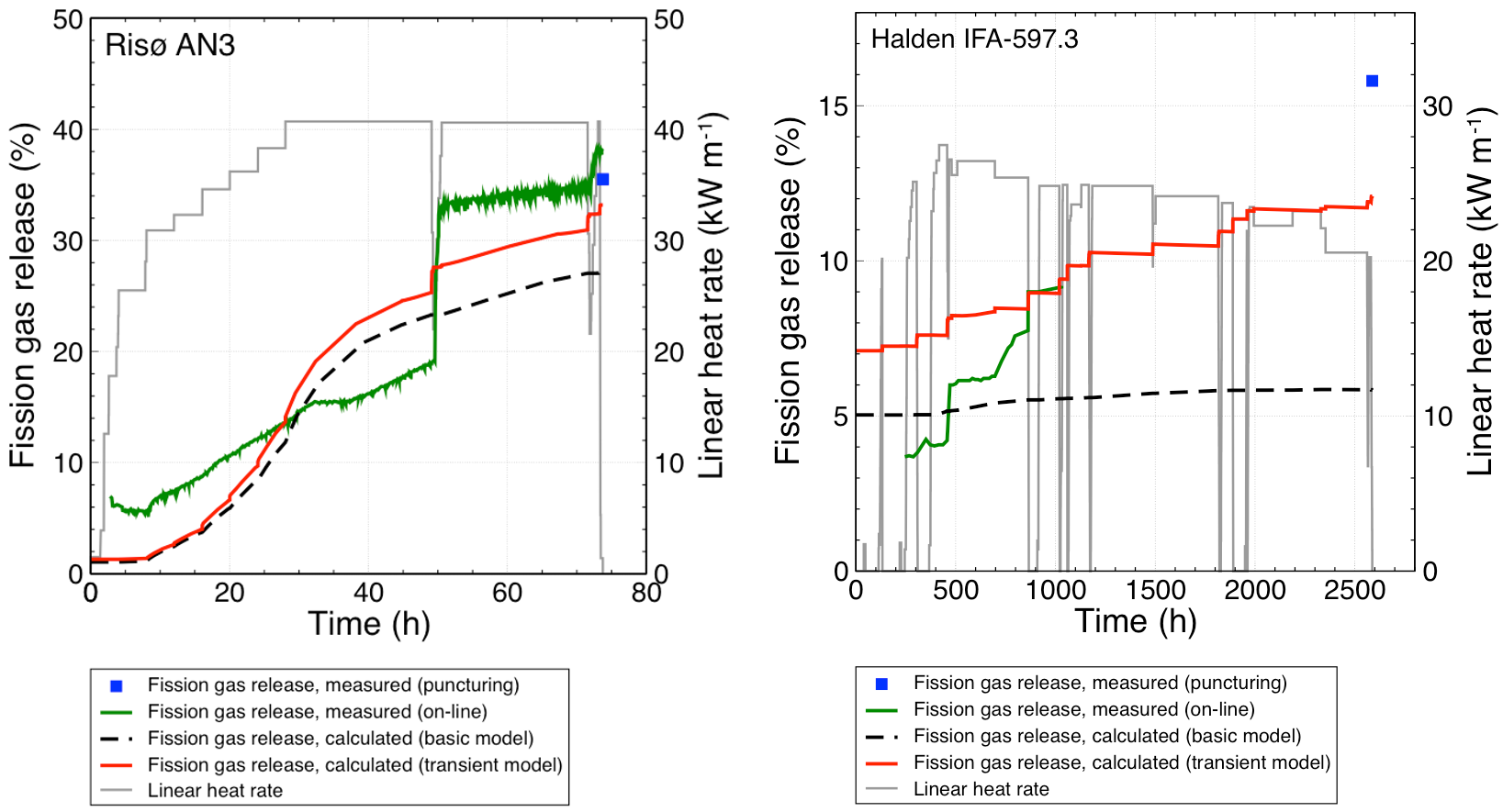
Current results are state-of-the-art or better
Material Models that Depend on Irradiation or Power
Zirconium
Uranium Dioxide
Power Profiles
Radial power profile example:
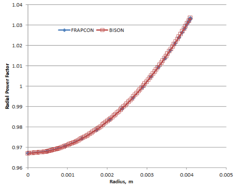
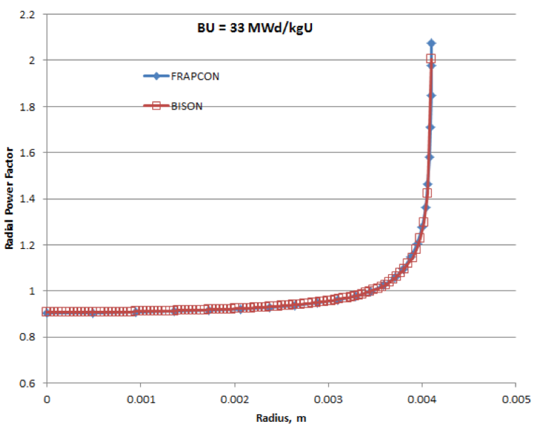
Don't forget the axial profile.
LWR Gap Heat Transfer
In BISON, and are described using the form proposed by Ross and Stoute (1962). is defined as
where is the conductivity of the gas in the gap, is the gap width, is a roughness coefficient, and are roughnesses of the surfaces, and and are jump distances, which become important for small gap widths and low gas pressures. The jump distances provide a reduction in gap conductance when the mean free path of the gas molecules is significant in comparison to the gap width, and the continuum approximation is no longer valid. The gas temperature () is the average of the two surfaces.
LWR Gap Heat Transfer
is defined as
where is an empirical constant, and are the thermal conductivities of the two materials, is the contact pressure, is the average gas film thickness, and is the Meyer hardness of the softer material.
LWR Gap Heat Transfer
In BISON, is computed using a diffusion approximation. Based on the Stefan-Boltzmann law,
where is the Stefan-Boltzmann constant, is an emissivity function, and and are the temperatures of the radiating surfaces.
The radiant conductance is approximated as
which can be reduced to
For infinite parallel plates,
where and are the emissivities of the radiating surfaces. This is the specific function implemented in BISON.
Example Problem
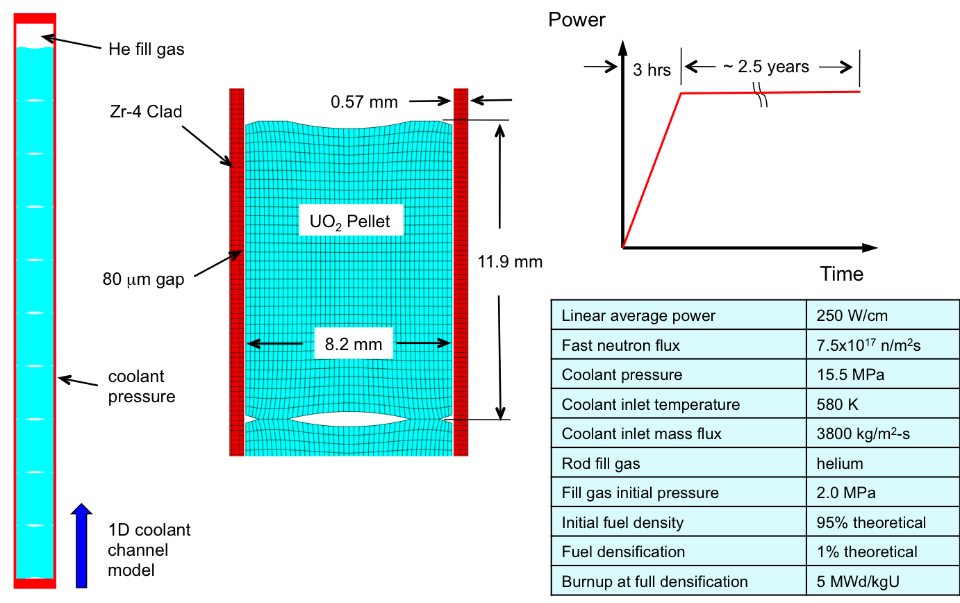
Axisymmetric 10 Pellet LWR Fuel Rodlet
Overview of the Example Problem
In this section, we will review the syntax found in an example problem.
The full input file is at
~/projects/bison/workshop/bison_example/Discrete.iThe input file syntax consists of blocks where the PDEs you are solving are defined.
High-level Description of the Input File
The input file is the place where you specify all the terms of your PDE(s) and supporting information to solve them. This is a different mindset than that used when running other simulation software.
Things you define here are:
Mesh
Global parameters (density and FE specification)
Coordinate system (RZ)
Physics kernels (individual terms in the PDE you're solving)
Source term (power)
Boundary conditions (convection coefficient and displacement BCs)
Material models (e.g., and Zr)
AuxKernels – Auxiliary equations that you want to solve that may be used as input to Kernels or BCs or just for visualization
Postprocessors (plenum pressure and average power)
What's the minimum input file content requirement for running a problem? That depends on what PDE(s) you are solving and the information needed to support those solves.
BISON Conventions
BISON uses several empirical models developed with a certain set of units.
BISON converts from the input units to the units needed by each empirical model.
The input units for BISON are:
meter, kilogram, second, kelvin, mole
BISON uses FIMA (fissions per initial metal atom) to describe burnup.
The coordinate convention for LWR analysis is that the rod axis corresponds to the y-axis in the global coordinate system. For axisymmetric RZ analyses, this implies that the r-direction (radial direction) corresponds to the x-axis and the z-direction corresponds to the y-axis.
BISON also includes several semi-empirical and mechanistically (lower length scale) informed models.
Common Kernels
Kernels often found in a BISON input file include:
HeatConduction
Gradient term in heat conduction equation
HeatConductionTimeDerivative
Time term in heat conduction equation
NeutronHeatSource
Source term in heat conduction equation
ArrheniusDiffusion
Arrhenius equation for mass diffusion
HeatSource
General source term for heat conduction or mass diffusion. For example, this could be used as an alternative to NeutronHeatSource.
Gravity
Decay
Sink term for mass diffusion or heat conduction
Common AuxKernels
AuxKernels often found in a BISON input file include:
FastNeutronFluxAux
Compute fast flux based on power
FastNeutronFluenceAux
Compute fast fluence based on fast flux
MaterialTensorAux
Compute volume-averaged stress and strain
FissionRateAux
Compute fission rate based on power
Not used if the Burnup block is used
BurnupAux
Compute burnup based on fission rate
This is not the same as the Burnup block
Not used if the Burnup block is used
Common Materials
Materials often found in a BISON input include:
UO2Thermal
Compute thermal conductivity and specific heat for fuel
HeatConductionMaterial
Set thermal conductivity and specific heat for a general material
Density
Compute density, which may change due to deformation
UO2CreepUpdate
Creep model for fuel
ZryCreepLimbackHoppeUpdate
Primary and secondary thermal and irradiation creep model for clad
UO2VolumetricSwellingEigenstrain
Densification and solid and gaseous swelling for fuel clad
UO2RelocationEigenstrain
Relocation model for fuel
UO2Sifgrs
Fission gas release model. Also has an option for calculating gaseous swelling.
Note that some of these models are empirical and have limited ranges of applicability.
Common BCs
BCs often found in a BISON input file include:
DirichletBC
FunctionDirichletBC
Set Dirichlet BCs based on a function
NeumannBC
Set gradient of a variable
Pressure
Set pressure on a surface
Note that this block requires sub-blocks
PlenumPressure
Set pressure on interior of clad, exterior of fuel
Note that this block requires subblocks
Common Postprocessors
Postprocessors often found in a BISON input file include:
SideAverageValue
Compute the area-weighted average of a variable
InternalVolume
Compute the volume of a closed sideset
SideDiffusiveFluxIntegral
Integrated flux over an area
TimestepSize
Report the time step size
ElementIntegralPower
Total power by integrating the fission rate over all elements
FunctionValuePostprocessor
Value of a time-varying function
Other Common Blocks
Other blocks often found in a BISON input file include:
Burnup
Compute the fission rate and burnup, including the radial power profile effect
Note that this block requires sub-blocks
Contact
Enforce mechanical contact constraints
Note that this block requires sub-blocks
ThermalContact
Enforce gap heat transfer
Note that this block requires sub-blocks
Physics/SolidMechanics/QuasiStatic
Divergence of stress in Cauchy's equation
Appears as its own block outside of Kernels
CoolantChannel
Compute a convective boundary condition for the clad
Note that this block requires sub-blocks
Executioner
Specify solver options and time-stepping controls
Outputs
Specify output options
Input Syntax
If you have questions about input syntax or what options are available for parameters.
Type:
~/projects/bison/bison-opt --dump
Example:
~/projects/bison/bison-opt --dump Postprocessors
Or use the Atom text editor, which supports MOOSE/BISON auto-completion and input syntax options.
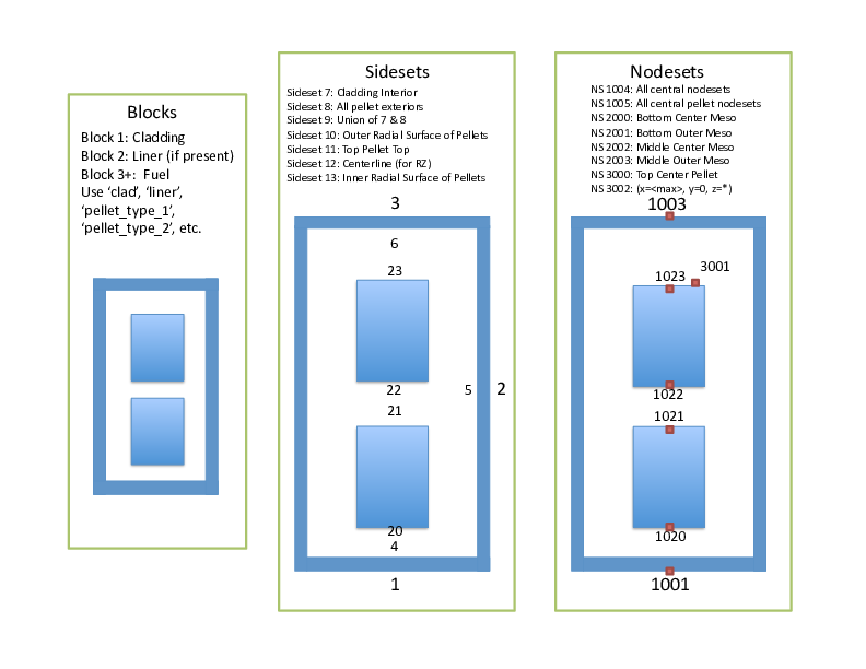
Blocks, sidesets, and nodesets
Some conventions to keep in mind as you look at the input file and consider blocks, sidesets, and nodesets in reference to BCs, source terms, and material models.
The GlobalParams Block
The GlobalParams block sets parameters that can be used by any other block. We can set parameters here instead of setting them over and over again in the remainder of the file. Here, we set the value of density, initial porosity, displacement solution variables, and variable order and family. The GlobalParams contains them, and so they are not needed in the Variables block. The GlobalParams block is often listed first, but can occur anywhere within the input file.
[GlobalParams]
  density = 10431.0
  initial_porosity = 0.05
  order = SECOND
  family = LAGRANGE
  energy_per_fission = 3.2e-11 # J/fission
  volumetric_locking_correction = true
  displacements = 'disp_x disp_y'
[]
The Problem Block
This block needs to be included for an axisymmetric analysis. It tells BISON that all of the boundary conditions, kernels, and material models should be evaluated in axisymmetric coordinates. Similarly coord_type can be set to RSPHERICAL to specify a 1D spherically symmetric analysis. type = ReferenceResidualProblem defines an alternative to evaluating convergence by converging each variable to its individual residual contribution contained in extra_vector_tags and reference_vector.
[Problem]
  type = ReferenceResidualProblem
  reference_vector = 'ref'
  extra_tag_vectors = 'ref'
[]
The Mesh Block
Mesh parameters are defined in this block. The following parameters are defined in this particular block:
file: defines the name of the finite element mesh file.displacements: lists the names of the displacement variables (needed for large displacement, contact). Note this was defined in the[GlobalParams]block.patch_size: used by contact to define the number of nearest neighbor nodes.partitioner: defines how the mesh is partitioned for parallel execution.
BISON also includes capability to build simple meshes (e.g., smeared pellet) from within the input file.
[Mesh]
  coord_type = RZ
  patch_update_strategy = always
  patch_size = 100 # For contact algorithm
  partitioner = centroid
  centroid_partitioner_direction = y
  [file]
    file = discrete.e
    type = FileMeshGenerator
  []
[]
The Variables Block
Dependent variables and initial conditions are examples of parameters defined in the variables block. Notice there are sub-blocks, whose names correspond to the dependent variables. Note that the displacement variables are not shown here. They are created by an Action that will be described later.
[Variables]
  [temp]
    initial_condition = 293.0
  []
[]
The AuxVariables Block
What are AuxVariables? They are variables in addition to the primary variables that allow explicit calculations. These can be used by kernels, boundary conditions, and material properties. AuxVariables are written to the output file. You can define two types of AuxVariables: Element (constant monomial) or Nodal (linear Lagrange). AuxVariables have old states, just like the primary variables. Some parameters you can set in this block are order (e.g., linear), family (e.g., Lagrange), and block. The block specifies on which blocks of the finite element mesh the named AuxVariable will be defined.
[AuxVariables]
  [fast_neutron_flux]
    block = clad
  []
  [fast_neutron_fluence]
    block = clad
  []
  [grain_radius]
    block = pellet_type_1
    initial_condition = 10e-6
  []
  [radial_strain]
    order = CONSTANT
    family = MONOMIAL
  []
  [effective_creep_strain]
    block = clad
    order = CONSTANT
    family = MONOMIAL
  []
  [gap_cond]
    order = CONSTANT
    family = MONOMIAL
  []
  [coolant_htc]
    order = CONSTANT
    family = MONOMIAL
  []
[]
The Functions Block
Functions can be used to define inputs to the simulation, such as power history, power factors, and pressure boundary conditions, to name a few. Notice some of the parameters you can specify, such as type (defines the function type), data_file (specifies the name of a data file), or value (sets the value of the function).
[Functions]
  [power_history]
    type = PiecewiseLinear
    data_file = powerhistory.csv
    scale_factor = 1
  []
  [axial_peaking_factors]
    type = PiecewiseBilinear
    data_file = peakingfactors.csv
    scale_factor = 1
    axis = 1 # (0,1,2) => (x,y,z)
  []
  [pressure_ramp]
    type = PiecewiseLinear
    x = '-200 0'
    y = '0 1'
  []
[]
A note about Actions
Here is a unique block entitled Physics/SolidMechanics/QuasiStatic.
This block defines the kernels relative to stress divergence, the displacement solution variables, and quantities of interest for output (stresses, strains, etc.). It has its own block to cut down on redundancy in the input file. Such a block is built using Actions from MOOSE. Future development work includes removing the requirement to specify any kernels for a typical fuels problem (because they are the same every time) and only specifying the unique parameters for a particular simulation.
[Physics]
  [SolidMechanics]
    [QuasiStatic]
      [pellets]
        block = pellet_type_1
        add_variables = true
        strain = FINITE
        eigenstrain_names = 'fuel_relocation_strain
                         fuel_thermal_strain
                         fuel_volumetric_strain'
        generate_output = 'vonmises_stress stress_xx
                       stress_yy stress_zz'
        extra_vector_tags = 'ref'
      []
      [clad]
        block = clad
        add_variables = true
        strain = FINITE
        eigenstrain_names = 'clad_thermal_eigenstrain
                         clad_irradiation_strain'
        generate_output = 'vonmises_stress stress_xx
                       stress_yy stress_zz'
        extra_vector_tags = 'ref'
      []
    []
  []
[]
The Kernels Block
Recall that kernels are used to define the various terms in the PDE set that you are solving. Each kernel is a term in the PDE. For example, the kernel gravity is the body force term in the stress divergence equation, heat is the gradient term in the heat conduction equation, heat_ie is the time term, and heat_source is the source term. Note that heat_source is connected to burnup (a Function) and applied only in the block pellet_type_1 (the fuel). The required parameters are type (the actual name of the kernel) and variable (temperature or displacement).
[Kernels]
  [gravity]
    type = Gravity
    variable = disp_y
    value = -9.81
  []
  [heat]
    type = HeatConduction
    variable = temp
    extra_vector_tags = 'ref'
  []
  [heat_ie]
    type = HeatConductionTimeDerivative
    variable = temp
    extra_vector_tags = 'ref'
  []
  [heat_source]
    type = NeutronHeatSource
    variable = temp
    extra_vector_tags = 'ref'
    block = pellet_type_1
    burnup_function = burnup
  []
[]
The Burnup Block
The Burnup block supplies input for computing burnup and fission rate based on the power history, the axial profile, and a radial power factor. The radial power factor is computed at grid points independent of the finite element mesh. The density of these points can be controlled with the num_radial and num_axial parameters. The parameters N235 through RPF are optional and specify that the associated isotope concentrations and radial power factor value should be written to the results file. The parameter i_enrich specifies the initial enrichment of the fuel.
[Burnup]
  [burnup]
    block = pellet_type_1
    rod_ave_lin_pow = power_history
    axial_power_profile = axial_peaking_factors
    num_radial = 80
    num_axial = 11
    a_lower = 0.00324 # mesh dependent!
    a_upper = 0.12184 # mesh dependent!
    fuel_inner_radius = 0
    fuel_outer_radius = .0041
    fuel_volume_ratio = 0.987775
    RPF = RPF
    # N235 = N235
    # N236 = N236
    # N238 = N238
    # N239 = N239
    # N240 = N240
    # N241 = N241
    # N242 = N242
  []
[]
The AuxKernels Block
The AuxKernels block defines the calculations to be performed for every AuxVariable. Important parameters include type (the kind of AuxKernel), variable (the AuxVariable to use), block (gives which mesh block the AuxKernel acts on), and execute_on, which specifies at which point in the algorithm the AuxKernel executes.
[AuxKernels]
  [fast_neutron_flux]
    type = FastNeutronFluxAux
    variable = fast_neutron_flux
    block = clad
    rod_ave_lin_pow = power_history
    axial_power_profile = axial_peaking_factors
    factor = 3e13
    execute_on = timestep_begin
  []
  [fast_neutron_fluence]
    type = FastNeutronFluenceAux
    variable = fast_neutron_fluence
    block = clad
    fast_neutron_flux = fast_neutron_flux
    execute_on = timestep_begin
  []
  [grain_radius]
    type = GrainRadiusAux
    block = pellet_type_1
    variable = grain_radius
    temperature = temp
    execute_on = linear
  []
  [radial_strain]
    type = RankTwoAux
    rank_two_tensor = total_strain
    variable = radial_strain
    index_i = 0
    index_j = 0
    execute_on = timestep_end
  []
  [effective_creep_strain]
    type = MaterialRealAux
    property = effective_creep_strain
    variable = effective_creep_strain
    block = clad
    execute_on = timestep_end
  []
  [conductance]
    type = MaterialRealAux
    property = gap_conductance
    variable = gap_cond
    boundary = 10
    execute_on = 'linear'
  []
  [coolant_htc]
    type = MaterialRealAux
    property = coolant_channel_htc
    variable = coolant_htc
    boundary = 2
    execute_on = 'linear'
  []
[]
Contact
The Contact block defines mechanical contact between the fuel (side set 10, secondary) and the clad (side set 5, primary).
penaltyis the stiffness of a constraint that prevents the surfaces from penetrating by applying a normal force along the contact surface.The thermal contact block specifies contact between the fuel (side set 10) and the clad (side set 5). The temperature variable must be given.
initial_molescouples to a Postprocessor that supplies the initial plenum/gap gas mass, andgas_releasedcouples to a Postprocessor that supplies the fission gas addition to the gap thermal conductance equation. More on Postprocessors later.
[Contact]
  [pellet_clad_mechanical]
    primary = 5
    secondary = 10
    formulation = kinematic
    model = frictionless
    penalty = 1e7
  []
[]

[ThermalContact]
  [thermal_contact]
    type = GasGapHeatTransfer
    variable = temp
    primary = 5
    secondary = 10
    initial_moles = initial_moles
    gas_released = fis_gas_released
    contact_pressure = contact_pressure
    quadrature = true
  []
[]
The Boundary Conditions Block
The
BCsblock describes thermal and mechanical boundary conditions applied to the mesh. For mechanics, rigid body motion must be prevented, which is achieved by theDirichletBCboundary conditions.The
Pressureboundary condition defines the coolant pressure. Notice the parameterfunctionthat refers to a function defined in the Functions block. The parameterfactorscales the pressure ramp function to complete the specification of pressure on the clad exterior.The
PlenumPressureblock defines the pressure on the inside of the clad and the outside of the fuel using the ideal gas law.initial_pressuresets the value of the fill gas pressure.Ris the universal gas constant. The other parameters are links to Postprocessors that provide input to this boundary condition. The parameteroutputwrites the magnitude of the plenum pressure to a Postprocessor calledplenum_pressure.
[BCs]
  [no_x_all]
    type = DirichletBC
    variable = disp_x
    boundary = 12
    value = 0.0
  []
  [no_y_clad_bottom]
    type = DirichletBC
    variable = disp_y
    boundary = '1'
    value = 0.0
  []
  [no_y_fuel_bottom]
    type = DirichletBC
    variable = disp_y
    boundary = '1020'
    value = 0.0
  []
  [Pressure]
    [coolantPressure]
      boundary = '1 2 3'
      factor = 15.5e6
      function = pressure_ramp
    []
  []
  [PlenumPressure]
    [plenumPressure]
      boundary = 9
      initial_pressure = 2.0e6
      startup_time = 0
      R = 8.3145
      output_initial_moles = initial_moles
      temperature = ave_temp_interior
      volume = gas_volume
      material_input = fis_gas_released
      output = plenum_pressure
    []
  []
[]
The Coolant Channel Block
This block specifies the convection of the coolant on the outside of the clad. boundary defines the side sets where the BC is applied. In this BC, inlet temperature, pressure, and mass flux are required. Rod diameter and pitch are also needed. Finally, the time-varying power profile and axially varying factors are given.
[CoolantChannel]
  [convective_clad_surface]
    boundary = '1 2 3'
    variable = temp
    inlet_temperature = 580 # K
    inlet_pressure = 15.5e6 # Pa
    inlet_massflux = 3800 # kg/m^2-sec
    rod_diameter = 0.948e-2 # m
    rod_pitch = 1.26e-2 # m
    linear_heat_rate = power_history
    axial_power_profile = axial_peaking_factors
  []
[]
The Material Properties/Models Block
The Materials block defines the thermal and mechanical behavior models and properties defined for the fuel and clad. The thermal models for are functions of temperature and burnup. The mechanics models specify features such as elasticity, creep, volumetric strains, fuel relocation, and clad growth. Note that many of the models are coupled to the primary and auxiliary variables as well as functions.
[Materials]
  [fuel_thermal]
    type = UO2Thermal
    block = pellet_type_1
    thermal_conductivity_model = NFIR
    temperature = temp
    burnup_function = burnup
  []
  [fuel_elasticity_tensor]
    type = ComputeIsotropicElasticityTensor
    block = pellet_type_1
    youngs_modulus = 2.0e11
    poissons_ratio = 0.345
  []
  [fuel_elastic_stress]
    type = ComputeFiniteStrainElasticStress
    block = pellet_type_1
  []
  [fuel_thermal_expansion]
    type = ComputeThermalExpansionEigenstrain
    block = pellet_type_1
    thermal_expansion_coeff = 10.0e-6
    temperature = temp
    stress_free_temperature = 295.0
    eigenstrain_name = fuel_thermal_strain
  []
  [fuel_relocation]
    type = UO2RelocationEigenstrain
    block = pellet_type_1
    burnup_function = burnup
    rod_ave_lin_pow = power_history
    axial_power_profile = axial_peaking_factors
    diametral_gap = 160.0e-6
    diameter = 0.0082
    burnup_relocation_stop = 0.035
    relocation_activation1 = 5000
    relocation_model = ESCORE_modified
    eigenstrain_name = fuel_relocation_strain
  []
  [fuel_volumetric_swelling]
    type = UO2VolumetricSwellingEigenstrain
    gas_swelling_model_type = SIFGRS
    block = pellet_type_1
    temperature = temp
    burnup_function = burnup
    initial_fuel_density = 10431.0
    eigenstrain_name = fuel_volumetric_strain
  []

  [clad_thermal]
    type = HeatConductionMaterial
    block = clad
    thermal_conductivity = 16.0
    specific_heat = 330.0
  []
  [clad_elasticity_tensor]
    type = ZryElasticityTensor
    block = clad
  []
  [clad_stress]
    type = ComputeMultipleInelasticStress
    tangent_operator = elastic
    inelastic_models = 'clad_zrycreep'
    block = clad
  []
  [clad_zrycreep]
    type = ZryCreepLimbackHoppeUpdate
    block = clad
    temperature = temp
    fast_neutron_flux = fast_neutron_flux
    fast_neutron_fluence = fast_neutron_fluence
    model_irradiation_creep = true
    model_primary_creep = true
    model_thermal_creep = true
    zircaloy_material_type = stress_relief_annealed
  []
  [thermal_expansion]
    type = ZryThermalExpansionMATPROEigenstrain
    block = clad
    temperature = temp
    stress_free_temperature = 295.0
    eigenstrain_name = clad_thermal_eigenstrain
  []
  [irradiation_swelling]
    type = ZryIrradiationGrowthEigenstrain
    block = clad
    fast_neutron_fluence = fast_neutron_fluence
    zircaloy_material_type = stress_relief_annealed
    eigenstrain_name = clad_irradiation_strain
  []
  [fission_gas_release]
    type = UO2Sifgrs
    block = pellet_type_1
    temperature = temp
    burnup_function = burnup
    grain_radius = grain_radius
    gbs_model = true
  []
  [clad_density]
    type = StrainAdjustedDensity
    block = clad
    strain_free_density = 6551.0
  []
  [fuel_density]
    type = StrainAdjustedDensity
    block = pellet_type_1
    strain_free_density = 10431.0
  []
[]
The Executioner
This block contains solver and time-stepping controls. The most important parameters are start_time, dt (time step), end_time, and the adaptive time-stepping options. The start time is set to -200, which accounts for the rise from cold zero to hot zero power (fabrication conditions to hot zero power reactor conditions).
[Executioner]
  type = Transient
  solve_type = 'PJFNK'

  petsc_options = '-snes_ksp_ew'
  petsc_options_iname = '-pc_type -pc_factor_mat_solver_package'
  petsc_options_value = 'lu       superlu_dist'

  line_search = 'none'

  l_max_its = 50
  l_tol = 8e-3
  nl_max_its = 15
  nl_rel_tol = 1e-4
  nl_abs_tol = 1e-10
  start_time = -200
  n_startup_steps = 1
  end_time = 8.0e7
  dtmax = 1e6
  dtmin = 1

  [TimeStepper]
    type = IterationAdaptiveDT
    dt = 2e2
    optimal_iterations = 8
    iteration_window = 2
    linear_iteration_ratio = 100
    growth_factor = 2
    cutback_factor = .5
  []
  [Quadrature]
    order = FIFTH
    side_order = SEVENTH
  []
[]
The Postprocessors Block
The Postprocessors block defines several quantities used throughout the simulation. This particular Postprocessor computes the average temperature of the cladding and all pellet exteriors. The result of a Postprocessor calculation is one scalar at every time step throughout the simulation. Recall that ave_temp_interior is used in the plenum pressure BC. There are too many to list, but here are the names of a few you will find in the example problem: fission_gas_produced, fission_gas_released, pellet_volume, and avg_clad_temp.
[Postprocessors]
  [ave_temp_interior]
    type = SideAverageValue
    boundary = 9
    variable = temp
    execute_on = 'initial linear'
  []
  [clad_inner_vol]
    type = InternalVolume
    boundary = 7
    execute_on = 'initial timestep_end'
  []
  [pellet_volume]
    type = InternalVolume
    boundary = 8
    execute_on = 'initial timestep_end'
  []
  [avg_clad_temp]
    type = SideAverageValue
    boundary = 7
    variable = temp
    execute_on = 'initial timestep_end'
  []
  [fis_gas_produced]
    type = ElementIntegralFisGasGeneratedSifgrs
    block = pellet_type_1
    execute_on = 'linear'
  []
  [fis_gas_released]
    type = ElementIntegralFisGasReleasedSifgrs
    block = pellet_type_1
    execute_on = 'linear'
  []
  [fis_gas_grain]
    type = ElementIntegralFisGasGrainSifgrs
    block = pellet_type_1
    outputs = exodus
    execute_on = 'linear'
  []
  [fis_gas_boundary]
    type = ElementIntegralFisGasBoundarySifgrs
    block = pellet_type_1
    outputs = exodus
    execute_on = 'linear'
  []
  [fission_gas_release]
    type = FGRPercent
    fission_gas_released = fis_gas_released
    fission_gas_generated = fis_gas_produced
    execute_on = 'linear'
  []
  [gas_volume]
    type = InternalVolume
    boundary = 9
    execute_on = 'initial linear'
  []
  [flux_from_clad]
    type = SideDiffusiveFluxIntegral
    variable = temp
    boundary = 5
    diffusivity = thermal_conductivity
  []
  [flux_from_fuel]
    type = SideDiffusiveFluxIntegral
    variable = temp
    boundary = 10
    diffusivity = thermal_conductivity
  []
  [rod_total_power]
    type = ElementIntegralPower
    variable = temp
    burnup_function = burnup
    block = pellet_type_1
  []
  [rod_input_power]
    type = FunctionValuePostprocessor
    function = power_history
    scale_factor = 0.1186 # rod height
  []

  [num_lin_it]
    type = NumLinearIterations
  []
  [num_nonlin_it]
    type = NumNonlinearIterations
  []
  [tot_lin_it]
    type = CumulativeValuePostprocessor
    postprocessor = num_lin_it
  []
  [tot_nonlin_it]
    type = CumulativeValuePostprocessor
    postprocessor = num_nonlin_it
  []
  [alive_time]
    type = PerfGraphData
    section_name = Root
    data_type = TOTAL
  []

  [fuel_centerline_temp]
    type = NodalVariableValue
    variable = temp
    nodeid = 2369
  []
  [fuel_surface_mid_temp]
    type = NodalVariableValue
    variable = temp
    nodeid = 2887
  []
  [fuel_surface_ridge_temp]
    type = NodalVariableValue
    variable = temp
    nodeid = 2862
  []
  [clad_surface_temp]
    type = NodalVariableValue
    variable = temp
    nodeid = 7322
  []
  [penetration_mid]
    type = NodalVariableValue
    variable = penetration
    nodeid = 2887
  []
  [penetration_ridge]
    type = NodalVariableValue
    variable = penetration
    nodeid = 2862
  []
  [average_burnup]
    type = RodAverageBurnup
    burnup_function = burnup
  []
[]
Outputs... FINALLY!
The parameter file_base specifies the prefix of the output file name. If not given, the output file base name will be the base name of the input file. exodus = true defines the type of output file. perf_graph specifies whether or not the performance log should be printed. csv = true defines that a CSV file containing all of the Postprocessor values be output.
[Outputs]
  perf_graph = true
  exodus = true
  color = false
  csv = true
  [outfile_clad_radial_displacement]
    type = CSV
    execute_on = 'timestep_end'
  []
  [outfile_fuel_radial_displacement]
    type = CSV
    execute_on = 'FINAL'
  []
[]
Other Examples
You will find other examples of running BISON at
bison/examples.It may also be helpful to review assessment cases at
bison/assessment.
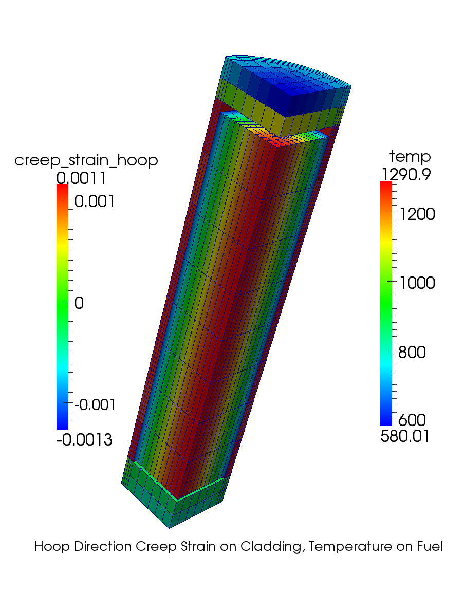
Other Materials for LWRs
While the preceding example showed how to setup a simple BISON model for and Zircaloy, BISON contains the capabilities to investigate other LWR materials.
USi fuel
CrO-doped
SiC-SiC cladding
FeCrAl cladding
Chromium-coated cladding
See bison/examples and the BISON documentation for further details.
Metallic Fuel Capabilities
Metallic Fuel-specific Models
In addition to the capability in MOOSE, BISON consists of:
Basic mechanics for the fuel and cladding
Elasticity
Plasticity
Creep
Thermal Conductivity
Fission gas release and swelling
Material models that are functions of irradiation
Creep
Thermal Conductivity
Gap heat transfer in sodium bond
Fuel-cladding chemical interaction (FCCI)
Zr redistribution
Fission Gas Behavior
EBR-II Experience
Zr redistribution with burnup
Different phases based on composition and temperature
Porosity shape and interconnection is phase dependent
Phases also depend on axial position (i.e., varying temperature and burnup)
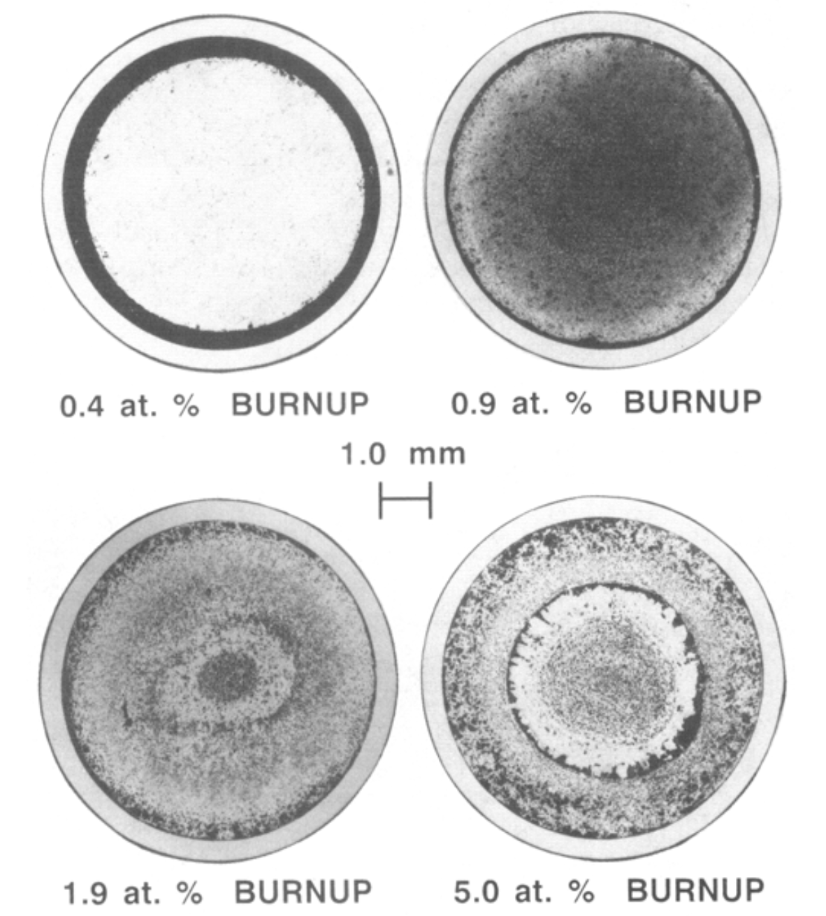
Fission Gas Behavior
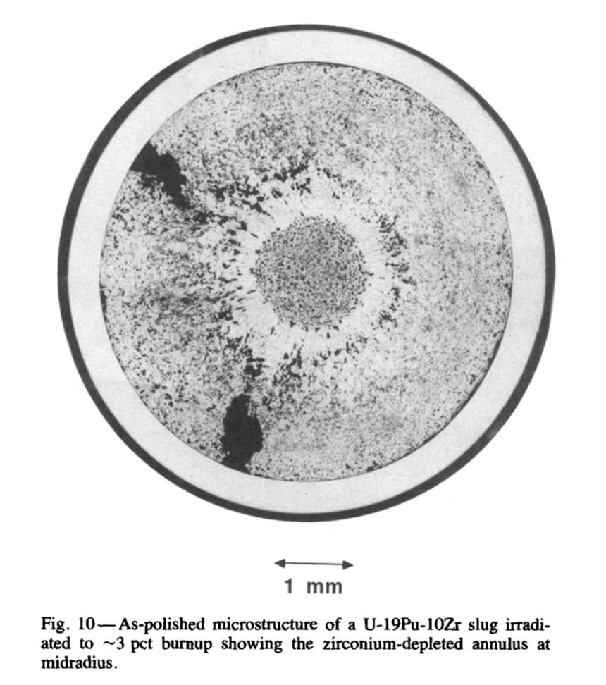
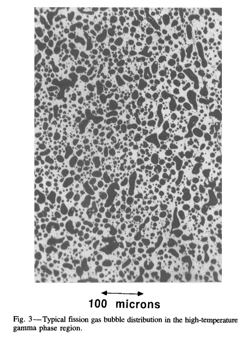
BISON Metallic Fuel Capabilities
General Capabilities
1.5D, 2D-RZ axisymmetric, and Cartesian 3D elements
Fully coupled thermo-mechanics and species diffusion
Strongly coupled
Loosely coupled
Linear and quadratic elements supporting large deformation
Steady and transient operation
EBR-II irradiations
TREAT experiments
Large-scale parallel computation
Desktop input preparation and syntax-checking
Actual input simulation on high performance clusters
Metallic Fuel Behavior
Both U-Zr and U-Pu-Zr
Able to specify weight percentage of binary or ternary fuel compositions
Temperature and species dependent conductivity
Anisotropic swelling
Thermal expansion
Irradiation-induced solid and gaseous swelling
Thermal and irradiation creep
Fission gas release (porosity-based)
Zr diffusion and redistribution
Gap and Plenum Behavior
Gap heat transfer (sodium conductivity)
Mechanical contact (primary and secondary)
Plenum pressure as a function of:
Evolving gas volume (from mechanics)
Gas mixture (from the fission gas release model)
Gas temperature approximation
Initial bond sodium volume above the fuel
Cladding Behavior
316 Stainless Steel, D9, and HT9
Mechanical properties including thermal expansion
Temperature dependent conductivity
Thermal and irradiation creep
Additional HT9 only models
Fuel-cladding chemical interaction (FCCI)
Cladding wastage thickness (burnup irradiations)
Basic eutectic thickness (transient over power events)
Failure (cumulative damage fraction) model
Coolant Channel
Closed-channel thermal hydraulics with heat transfer coefficients
Simple calculation of enthalpy rise of coolant with heat removal
Sodium fluid properties
Single-phase (liquid) correlations:
Triangular sub-channel (EBR-II assembly)
Tube within tube (TREAT experiment)
Assessments
Assessment cases are larger BISON input cases typically divided into two categories: benchmarks and validation.
For metallic fuel, the list of assessment cases completed thus far are available here.
Open Assessment Input
You've seen a few inputs.
Let's open an input in your favorite text editor.
Atom
Emacs
Vim
Notepad++
Practice identifying what the simulation will do.
Burnup and Transient Simulations
Burnup vs Transient
Burnup
Time scales of months to years
Gradual change to fuel composition
Slow or small changes to simulation inputs
Fission gas production
Not really "steady-state"
Transient
Time scales of usually less than a week
Abrupt or quick changes to simulation inputs
"Off-normal" fuel conditions
Behavior may differ from burnup behavior
Traditionally more difficult to solve
What is the difference?
The first place to check is the
ExecutionerblockBurnup and Transient simulations are
type = Transient
[Executioner]
  type = Transient
  nl_rel_tol = 1e-6
  nl_abs_tol = 1e-9
  start_time = 0.0
  end_time = 1
  dtmin = 1e-6
  dtmax = 0.1

  [TimeStepper]
    type = ConstantDT
    dt = 0.01
  []
[]
What is the difference?
[Executioner]
  type = Transient
  nl_rel_tol = 1e-6
  nl_abs_tol = 1e-9
  start_time = 0.0
  end_time = 1
  dtmin = 1e-6
  dtmax = 0.1

  [TimeStepper]
    type = ConstantDT
    dt = 0.01
  []
[]
The
Executionerblock also contains time step information:Time step size
Time beginning
Time ending
Some simulations have initial ramps or cooldowns requiring a mix of small time steps and larger ones.
Some transients occur at the end of a base irradiation simulation.
TimeStepper
A TimeStepper is used to provide the time step size (
dt).Common TimeStepper types:
ConstantDTFunctionDTIterationAdaptiveDT
ConstantDTprovides a constantdt.FunctionDTprovides adtsize that depends on time.When a time step fails to converge,
dtis reduced, and the time step is tried again.Reduction ratio may be controlled.
Minimum allowable
dtmay be set.If minimum
dtfails to converge, the simulation exits at that time step.
IterationAdaptiveDT TimeStepper
The
IterationAdaptiveDTTimeStepper controls the time step based on the solution difficulty, measured by the number of iterations required to solve the previous step.It can also adjust the solution time, based on changes in a time-dependent function (i.e., power history).
Adjustments are usually made with both nonlinear and linear iteration amounts. The TimeStepper may be set to only use nonlinear iteration amount.
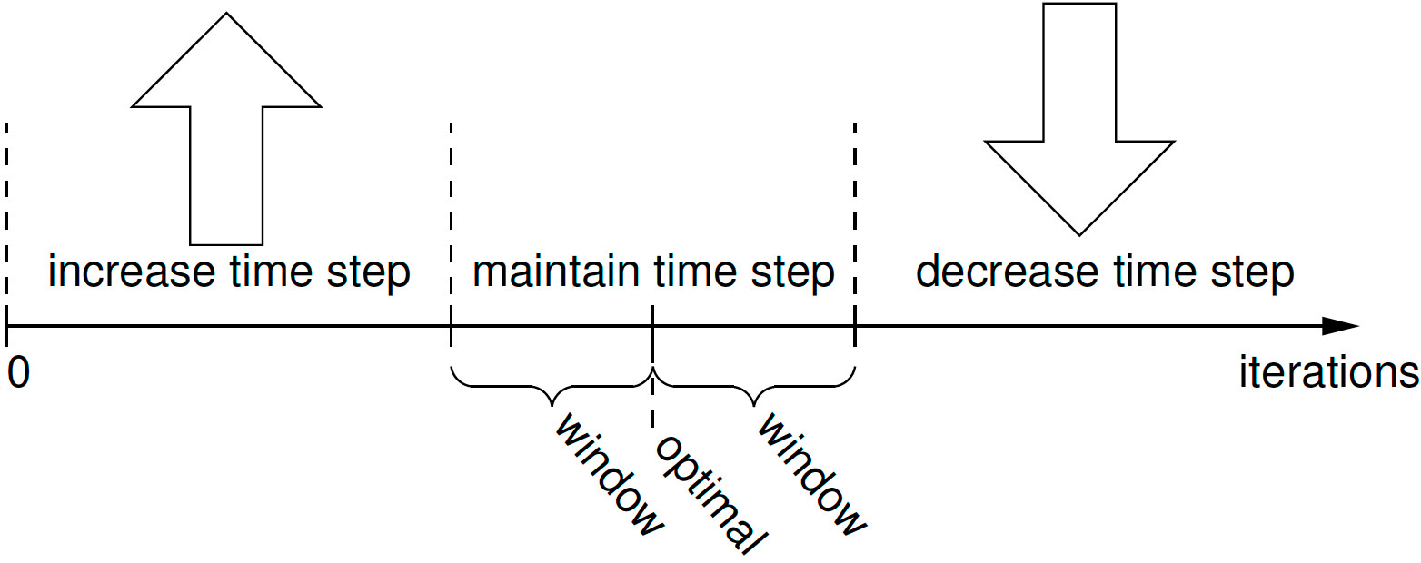
Check the Physics
The best place for checking what is actually going on is the
Kernelsblock.
[Kernels]
  [heat]
    type = HeatConduction
    variable = T
  []
  [heat_ie]
    type = HeatConductionTimeDerivative
    variable = T
  []
  [heat_source_right]
    type = HeatSource
    block = 0 # left
    variable = T
    function = left_heat
  []
[]
Quasi-Transient
Uses the transient executioner, but there are no
TimeDerivativekernels.Useful for coupled physics when one physics reacts much more quickly than the other coupled physics during the same time period.
- The slower physics (e.g., no waves, inertial effects) is approximated as quasi-static by not including a time derivative.
- The remaining coupled physics still include time derivatives producing a a coupled quasi-transient simulation.
MOOSE's modular approach to physics makes this work simply by including kernels specific to the important physics of the problem.
Also true for material models.
Transient Solving to Steady State
Time evolution from the initial state to a steady state is desired.
Use "negative" time to bring simulation state to the required initial state.
At time = 0, change an input to begin the time evolution.
Only required if initial state is not easily set within BISON.
Transient executioner is used.
Able to detect when steady state occurs:
steady_state_detection = trueMay want to change
steady_state_tolerancevalue.
LWR Burnup
A burnup block action is used to set up the burnup system.
Actions have a documentation page: Burnup
Describes what blocks the action creates behind the scenes.
States what parameters are changed from their default values.
Shows example inputs.
Actions are usually documented in links from the section heading.
Click on the
Burnupheading in the documentation page.
Metallic Fuel Burnup
Burnup is handled differently for metallic fuel compared to LWR fuel.
Metallic fuel uses material model
UPuZrBurnupto compute burnup.Uses the
fission_ratematerial property.Fuel composition is also an input.
Material property created with the burnup value (default is
burnup).Use
outputs = allto also place burnup value in an AuxVariable.
Burnup material property may be set another way, if needed.
Postprocessors and VectorPostprocessors Overview
Postprocessors
Recall that Postprocessors return a single scalar value at each time step.
Throughout the training, you have been exposed to a variety of different Postprocessors. Let's review the complete list of Postprocessors available in BISON.
VectorPostprocessors (VPP)
VPPs are a specialization of a MOOSE UserObject that outputs a vector of scalar values at each time step.
These objects can be fed to the
Outputssystem to limit how often they are executed.In BISON, typical use cases for VPPs include:
Fuel and cladding radial profilometry
Radial temperature profiles
Radial burnup profiles
Let's review the complete list of VPPs available in MOOSE/BISON.
Building Input File Complexity
Overview
In this section, we explore MOOSE systems and capabilities that provide the user with significantly more control over their simulation analysis.
Topics explored include:
PiecewiseBilinear functions
Parsed functions
Generic function materials
Parsed materials
UserObjects
PiecewiseBilinear Functions
Piecewise bilinear functions have been used for the axial profile in nuclear fuel rods.
The format of this csv file is as follows:
| coor_1 | coor_2 | coor_3 | coor_M | ||
| time_1 | factor11 | factor12 | factor13 | factor1M | |
| time_2 | factor21 | factor22 | factor23 | factor2M | |
| time_N | factornN1 | factorN2 | factorN3 | factorNM |
Parsed Functions
Parsed functions allow the user to specify complicated functions that are a function of position (x,y,z) and time.
[Functions]
  [clad_displacement_function]
    type = ParsedFunction
    expression = '2.0e-5 * t * sin(pi * y / 0.5)'
  []
[]
Parsed functions can be a function of Postprocessor values.
[Functions]
  [heat_generation]
    #A factor to multiply the pulse history to get desired energy/gram into the fuel
    type = ParsedFunction
    expression = 'energy / (pi * fuelradius * fuelradius * height) / pulsewidth'
    symbol_names = 'height energy pulsewidth fuelradius'
    symbol_values = '0.1 zz_total_energy zz_FWMH zz_fuel_OR'
  []
[]
Parsed Functions (continued)
Parsed functions can define their own variables directly.
[Functions]
  [flux_exact_fcn]
    type = ParsedFunction
    symbol_names = 'linear_power axial_profile'
    symbol_values = 'linear_power axial_profile'
    expression = 'epf := 1 / pi / 10.0;
             rad_outer := 2;
             rad_inner := 1;
             ratio := 0.3;
             fsnrateden := ratio * linear_power * axial_profile / (rad_outer^2 - rad_inner^2) / pi / epf;
             U_ratio := 0.2;
             Pu_ratio := 0.3;
             X_Pu := 0.2;
             X_Zr := 0.1;
             X_U := 1.0 - X_Pu - X_Zr;
             X_U235 := X_U * U_ratio;
             X_U238 := X_U - X_U235;
             X_Pu240 := X_Pu * Pu_ratio;
             X_Pu239 := X_Pu - X_Pu240;
             A_U235 := 0.2350439231;
             A_U238 := 0.2380507826;
             A_Pu239 := 0.2390521565;
             A_Pu240 := 0.2400538075;
             A_Zr := 0.091224;
             Atot := X_U235 * A_U235 + X_U238 * A_U238 + X_Pu239 * A_Pu239 + X_Pu240 * A_Pu240 + X_Zr * A_Zr;
             sigma_U235 := 1.0e4;
             sigma_U238 := 1.0e3;
             sigma_Pu239 := 1.0e4;
             sigma_Pu240 := 8199.0380426;
             density := 4;
             Ntot := density * 6.022e23 * 1.0e-28 / Atot;
             sigma_tot := Ntot * (X_U235 * sigma_U235 + X_U238 * sigma_U238 + X_Pu239 * sigma_Pu239 + X_Pu240 * sigma_Pu240);
             fsnrateden / sigma_tot'
  []
[]
Parsed Functions (continued)
Parsed functions can depend on globally defined parameters.
# This test is used to verify the implementation of DiffusionLimitedReaction.
# The result is compared against the exact formulation of the diffusion limited
# reaction. Averaging of the values of the material properties  that formulate
# the rate in DiffusionLimitedReaction with the current and previous timestep values
# is compared against a fully implicit solve. The two methods are compared against
# the exact formulation. The damper can be tuned to provide closer answers to
# the exact formulation by forcing the timestep to drop.

tend = 1
rstart = 1e-5
rend = 1e-1
ic = 1e-2

[Mesh]
  [mesh]
    type = GeneratedMeshGenerator
    dim = 1
  []
[]

[Variables]
  [u]
    initial_condition = ${ic}
  []
  [v]
    initial_condition = ${ic}
  []
[]

[Kernels]
  [dt_u]
    type = TimeDerivative
    variable = u
  []
  [diff_rx_u]
    type = DiffusionLimitedReaction
    variable = u
    average_with_old = true
    radius = radius
    diffusivity = D
    sink_concentration = C_b
  []

  [dt_v]
    type = TimeDerivative
    variable = v
  []
  [diff_rx_v]
    type = DiffusionLimitedReaction
    variable = v
    average_with_old = false
    radius = radius
    diffusivity = D
    sink_concentration = C_b
  []
[]

[Functions]
  [u_exact]
    type = ParsedFunction
    symbol_names = 'radius_avg D_avg C_b_avg'
    symbol_values = 'radius_avg D_avg C_b_avg'
    expression = '${ic} *exp(-4 * pi * D_avg * C_b_avg * (${rstart} * ${tend} + 0.5 * (${rend} - ${rstart}) / ${tend} * t^2))'
  []
  [radius_ramp]
    type = PiecewiseLinear
    x = '0 ${tend}'
    y = '${rstart} ${rend}'
  []

  [u_error]
    type = ParsedFunction
    symbol_names = 'u_avg u_exact'
    symbol_values = 'u_avg u_exact'
    expression = '(u_exact - u_avg) / u_exact'
  []
  [v_error]
    type = ParsedFunction
    symbol_names = 'v_avg u_exact'
    symbol_values = 'v_avg u_exact'
    expression = '(u_exact - v_avg) / u_exact'
  []
[]

[Materials]
  [props]
    type = GenericFunctionMaterial
    prop_names = 'radius C_b D'
    prop_values = 'radius_ramp 1 1'
    outputs = all
  []
[]

[Dampers]
  [u]
    type = MaxIncrement
    increment_type = fractional
    variable = u
    max_increment = 1e-2
  []
  [v]
    type = MaxIncrement
    increment_type = fractional
    variable = v
    max_increment = 1e-2
  []
[]

[Executioner]
  type = Transient

  end_time = ${tend}

  [TimeStepper]
    type = IterationAdaptiveDT
    dt = 1e-3
  []
[]

[Postprocessors]
  [u_avg]
    type = ElementAverageValue
    variable = u
  []
  [v_avg]
    type = ElementAverageValue
    variable = v
  []
  [u_exact]
    type = FunctionValuePostprocessor
    function = u_exact
  []
  [radius_avg]
    type = ElementAverageValue
    variable = radius
  []
  [D_avg]
    type = ElementAverageValue
    variable = D
  []
  [C_b_avg]
    type = ElementAverageValue
    variable = C_b
  []
  [error_v]
    type = FunctionValuePostprocessor
    function = v_error
  []
  [error_u]
    type = FunctionValuePostprocessor
    function = u_error
  []
  [dt]
    type = TimestepSize
  []
[]

[Outputs]
  csv = true
[]
Generic Function Materials
Generic function materials are user-specified materials defined by functions within the input file rather than coding in C++.
Useful for users with no experience in coding, but who have a new material model.
All the details of the material are contained within the input file.
Generic Function Materials Example
# This test checks UPuZrFastNeutronFlux against a hand calculation while varying all possible input
# parameters.
#
# dpa should compute to 1 at the final timestep to ensure fluence and dpa are being calculated correctly

[Problem]
  solve = false
[]

[Mesh]
  coord_type = RZ
  [mesh]
    type = GeneratedMeshGenerator
    dim = 2
    nx = 1
    ny = 8
    ymax = 8
  []
[]

[Functions]
  [linear_power]
    type = ParsedFunction
    expression = 't'
  []
  [axial_profile]
    type = ParsedFunction
    expression = 'y'
  []
  [flux_exact_fcn]
    type = ParsedFunction
    symbol_names = 'linear_power axial_profile'
    symbol_values = 'linear_power axial_profile'
    expression = 'epf := 1 / pi / 10.0;
             rad_outer := 2;
             rad_inner := 1;
             ratio := 0.3;
             fsnrateden := ratio * linear_power * axial_profile / (rad_outer^2 - rad_inner^2) / pi / epf;
             U_ratio := 0.2;
             Pu_ratio := 0.3;
             X_Pu := 0.2;
             X_Zr := 0.1;
             X_U := 1.0 - X_Pu - X_Zr;
             X_U235 := X_U * U_ratio;
             X_U238 := X_U - X_U235;
             X_Pu240 := X_Pu * Pu_ratio;
             X_Pu239 := X_Pu - X_Pu240;
             A_U235 := 0.2350439231;
             A_U238 := 0.2380507826;
             A_Pu239 := 0.2390521565;
             A_Pu240 := 0.2400538075;
             A_Zr := 0.091224;
             Atot := X_U235 * A_U235 + X_U238 * A_U238 + X_Pu239 * A_Pu239 + X_Pu240 * A_Pu240 + X_Zr * A_Zr;
             sigma_U235 := 1.0e4;
             sigma_U238 := 1.0e3;
             sigma_Pu239 := 1.0e4;
             sigma_Pu240 := 8199.0380426;
             density := 4;
             Ntot := density * 6.022e23 * 1.0e-28 / Atot;
             sigma_tot := Ntot * (X_U235 * sigma_U235 + X_U238 * sigma_U238 + X_Pu239 * sigma_Pu239 + X_Pu240 * sigma_Pu240);
             fsnrateden / sigma_tot'
  []
[]

[Materials]
  [flux]
    type = UPuZrFastNeutronFlux
    axial_power_profile = axial_profile
    rod_linear_power = linear_power
    fast_spectrum_ratio = 0.3
    initial_X_Pu = 0.2
    initial_X_Zr = 0.1
    initial_density = 4
    pellet_inner_radius = 1.0
    pellet_radius = 2.0
    enrichment_Pu240 = 0.3
    enrichment_U235 = 0.2
    sigma_U235 = 1.0e4
    sigma_U238 = 1.0e3
    sigma_Pu239 = 1.0e4
    sigma_Pu240 = 8199.0380426
    energy_per_fission = 0.031830989
    dpa_conversion_factor = 1.9245015
    outputs = all
    calculate_fluence = true
    calculate_dpa = true
    calculate_dpa_rate = true
    fast_neutron_flux_name = 'asdf_fast_neutron_flux'
    fast_neutron_fluence_name = 'asdf_fast_neutron_fluence'
    dpa_name = 'asdf_dpa'
  []
  [flux_exact]
    type = GenericFunctionMaterial
    prop_names = 'flux_exact'
    prop_values = 'flux_exact_fcn'
    outputs = all
  []
[]

[Executioner]
  type = Transient
  num_steps = 2
[]

[Postprocessors]
  [flux_old]
    type = ElementAverageValue
    variable = asdf_fast_neutron_flux
    execute_on = 'TIMESTEP_BEGIN'
  []
  [flux_avg]
    type = ElementAverageValue
    variable = 'asdf_fast_neutron_flux'
  []
  [flux_exact_avg]
    type = ElementAverageValue
    variable = 'flux_exact'
  []
  [flux_error]
    type = ElementL2Error
    variable = asdf_fast_neutron_flux
    function = flux_exact_fcn
  []

  [dt]
    type = TimestepSize
  []
  [fluence_avg]
    type = ElementAverageValue
    variable = 'asdf_fast_neutron_fluence'
  []
  [dfluence_exact]
    type = ParsedPostprocessor
    pp_names = 'flux_avg flux_old dt'
    expression = 'dt * (flux_avg + flux_old) / 2'
  []
  [fluence_exact]
    type = CumulativeValuePostprocessor
    postprocessor = dfluence_exact
  []
  [fluence_diff]
    type = ParsedPostprocessor
    pp_names = 'fluence_avg fluence_exact'
    expression = '(fluence_avg - fluence_exact) / fluence_exact'
    outputs = console
  []
  [fluence_max_diff]
    type = TimeExtremeValue
    postprocessor = fluence_diff
    value_type = abs_max
  []

  [dpa_rate_avg]
    type = ElementAverageValue
    variable = 'asdf_dpa_rate'
  []
  [dpa_rate_exact]
    type = ParsedPostprocessor
    pp_names = 'flux_avg flux_old dt'
    expression = '(flux_avg + flux_old) / 2 / 1.9245015'
  []
  [dpa_rate_diff]
    type = ParsedPostprocessor
    pp_names = 'dpa_rate_avg dpa_rate_exact'
    expression = '(dpa_rate_avg - dpa_rate_exact) / dpa_rate_exact'
    outputs = console
  []
  [dpa_rate_max_diff]
    type = TimeExtremeValue
    postprocessor = dpa_rate_diff
    value_type = abs_max
  []

  [dpa_avg]
    type = ElementAverageValue
    variable = 'asdf_dpa'
  []
  [dpa_exact]
    type = CumulativeValuePostprocessor
    postprocessor = 'dpa_rate_exact'
  []
  [dpa_diff]
    type = ParsedPostprocessor
    pp_names = 'dpa_avg dpa_exact'
    expression = '(dpa_avg - dpa_exact) / dpa_exact'
    outputs = console
  []
  [dpa_max_diff]
    type = TimeExtremeValue
    postprocessor = dpa_diff
    value_type = abs_max
  []
[]

[Outputs]
  csv = true
[]
Parsed Materials
Parsed materials are another way to define complicated materials directly in the input file.
[Materials]
  [D_exact]
    type = ParsedMaterial
    property_name = D_exact
    coupled_variables = temp
    constant_names = 'Q1 D01 Q2 D02 R'
    constant_expressions = '0.5 5 0.1 3e-3 8.617e-5'
    expression = 'D01 * exp(-Q1 / R / temp) + D02 * exp(-Q2 / R / temp)'
    outputs = all
  []
[]
UserObjects
UserObjects are one of the more complicated but powerful systems in MOOSE.
UserObjects can be functions of material properties, functions, variables, AuxVariables, Postprocessors, and other UserObjects.
Unlike other systems in MOOSE/BISON, the developer must perform the correct parallelization.
Details of the UserObjects system can be found here.
UserObjects: Fuel Pin Geometries
In BISON, many material models depend upon the geometry of the mesh.
The FuelPinGeometry suite of UserObjects was developed to protect the user from potential input errors by automatically reading the geometric information from the mesh.
FuelPinGeometry objects available in BISON:
UserObjects: Terminator
The terminator UserObject allows the simulation to gracefully terminate when a Boolean expression containing a Postprocessor is achieved.
Useful during transient analyses (e.g., Loss of Coolant Accidents) when a cladding failure criteria is achieved.
When a certain burnup is achieved.
[UserObjects]
  [pin_geometry]
    type = Layered1DFuelPinGeometry
    mesh_generator = layered1D_mesh
  []
  [terminator1]
    type = Terminator
    expression = 'burnup_EAV >= 0.0632'
  []
  [terminator2]
    type = Terminator
    expression = 'plenum_pressure >= 1.55e7'
  []
[]
Submitting Issues
What is an Issue?
An issue is what is created on BISON's Enterprise GitHub site.
Used to report a defect or bug.
Used to suggest a feature or improvement of a feature.
Issues drive development and discussion.
Issue lists also show what BISON-related bugs or features are known to the developers.
Search the issues to avoid duplicating them.
Join discussions if you can add information to help the process along.
You can customize alerts to follow issues even without participating in them.
BISON Users Mailing List
We maintain a BISON users mailing list.
Everyone on the list gets an email.
When to email the users list:
Not sure if something really is an issue or not.
Still need help even after consulting documentation.
Unexpected behavior regarding BISON (e.g., installation, simulation results)
Clarification on documentation.
General discussion or BISON-related alerts all members should be aware of.
To get on the list, email any BISON developer, and we will add that email address to the list.
The same is true for getting off the list.
What We Need
When submitting an issue, choose a template from the list and fill it out correctly and fully.
Both issues and mailing list queries should have enough information for us to reproduce or understand the problem.
Commit hash of BISON
Operating system details (i.e., name, version)
An input, simplified input, or related input that produces the behavior, if possible. Remember that this is visible to all BISON users.
Complete log of simulation output, if possible.
WHY you are reaching out to us.
HOW you already tried to address the issue.
WHAT you expected to happen or want to happen.
Issue Creation
To Enterprise GitHub!
Contributing to BISON
Why Contribute
Many hands make light work.
Four eyes see more than two.
Two heads are better than one.
How to Contribute
Issues (Don't let them get swept under the rug.)
BISON user mailing list (you can answer other's questions, too.)
Documentation polishing (submit a merge request.)
Code additions and fixes (submit a merge request.)
Help out other BISON users in your local area. (And get help from them, too.)
Submitting a Merge Request
Merge Requests are equivalent to GitHub's "Pull Requests"
To start a merge request, you will need:
A personal fork of BISON.
An issue (new or old) submitted to
idaholab/bison.A branch on your fork containing the proposed changes in a single commit.
Merge Requests Requirements
The merge request must reference an open issue on
idaholab/bison.The merge request must pass an automatic check.
Check code and documentation build.
Check that regression tests have not changed.
Check that software quality requirements are met.
The merge request must pass a manual review.
A BISON developer will review and make comments about and within the merge request changes.
All comments must be resolved.
The BISON developer has the final say on what is merged into
idaholab/bison.
After merging, heavy test cases and assessment cases are checked over night to ensure they remain unchanged.
We appreciate you helping us out in the event your changes "break" something.
Merges can be reverted, though we prefer not to do that.
Location, Location, Location
Where does everything go?
srccontains*.Ccode.includecontains*.hheaders.doc/contentcontains*.mddocumentation files.test/testscontains regression tests and their "gold" outputs. The "test" file here contains the software quality requirements:issueslinks the test to an issue.designlinks the test to a documentation file.requirementdescribes what the test shall do.
Use other files as examples or ask a developer for help.
Merge requests can be opened as "Work In Progress".
Developers should be given access to your fork, allowing them to look at the changes made to your branch.
Merge Request Creation
To HPC Enterprise GitHub!
Sensitivity Analysis and
Uncertainty Quantification
Uncertainty Quantification
Uncertainty exists in numerical models, boundary conditions (e.g., power), geometry (due to manufacturing), and experimental measurements.
Traditionally, fuel performance modeling has not incorporated uncertainty into calculations.
The Best-Estimate Plus Uncertainty (BEPU) methodology has started to be adopted by the fuel performance modeling community.
Improved quantification of uncertainty in validation data obtained from experiments is crucial.
Direct propagation of uncertainty in inputs to quantify the uncertainty in output metrics of interest is known as "forward uncertainty quantification."
Sensitivity Analysis
Sensitivity analysis explores correlations between uncertain inputs and the output metrics of interest.
Insight can be gained into which uncertain inputs contribute the most to the uncertainty in a particular output metric.
BISON-Dakota Coupling
BISON has been coupled to Dakota to perform UQ and SA.
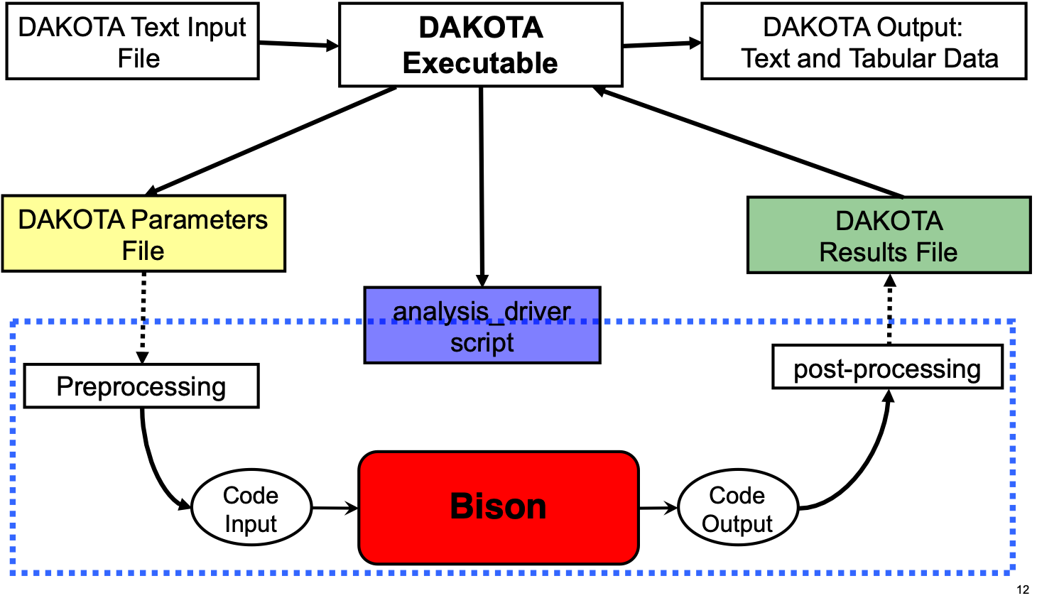
Example of UQ and SA on an Accident Tolerant Fuel Problem
Problem Description
Two USi-fueled experiments with ZIRLO cladding
Available data includes fission gas release, fuel stack elongation, and clad profilometry
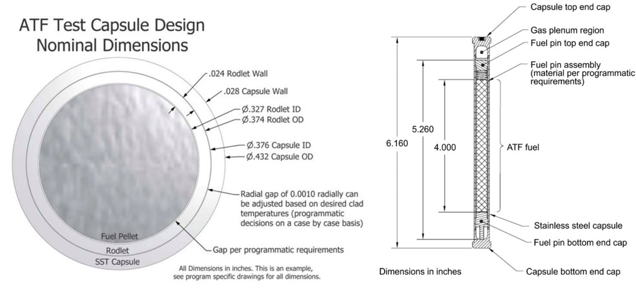
Barrett et al., Nuc. Eng. Des., 294, 38-51 (2015)
Uncertain Parameters
Select models for USi were chosen as uncertain inputs. A scaling factor corresponding to a 95% confidence interval was selected.
See milestone report for details on equation numbers.
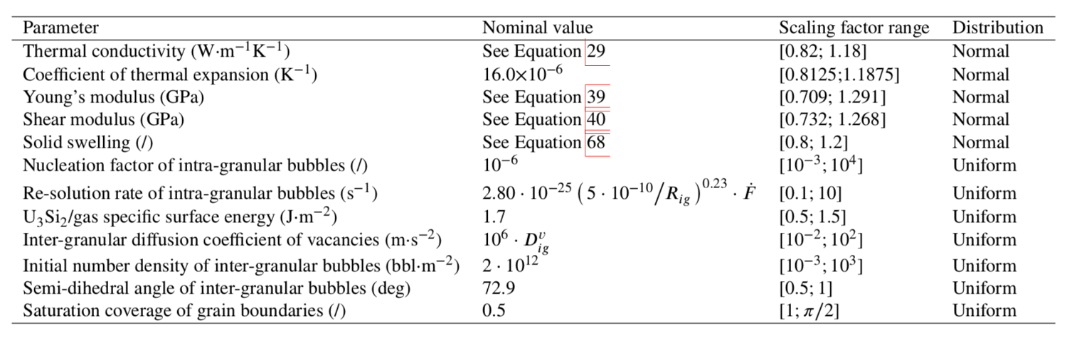
Dakota Input File
#  DAKOTA INPUT FILE

environment,
  tabular_graphics_data

method,
  sampling
  sample_type lhs
  samples = 480
  seed = 3487

model
  single

variables,
  active all
  uniform_uncertain = 4
    lower_bounds = 0.1 0.5 0.5 1.0
    upper_bounds = 10.0 1.5 1.0 1.570796327
    descriptors = 'resolution_rate' 'surface_energy' 'semi_dihedral_angle' 'saturation_coverage'

  loguniform_uncertain = 3
    lower_bounds = 10.0e-3 10.0e-2 10.0e-3
    upper_bounds = 10.0e4 10.0e2 10.0e3
    descriptors = 'nucleation_factor' 'inter_granular_diffusion' 'number_density'

  normal_uncertain = 5
    mean = 1.0 1.0 1.0 1.0 1.0
    std_deviations = 0.09 0.09375 0.1455 0.134 0.1
    lower_bounds = 0.82 0.8125 0.709 0.732 0.8
    upper_bounds = 1.18 1.1875 1.291 1.268 1.2
    descriptors = 'thermal_cond' 'thermal_expansion' 'youngs_modulus' 'shear_modulus' 'solid_swelling'

interface,
  system
   analysis_driver = 'run_submission'
   parameters_file = 'params.in'
   results_file    = 'results.out'
   file_save file_tag

responses,
  num_response_functions = 2
  descriptors = 'pellet_volume' 'fgr_perecent'
  no_gradients
  no_hessians
Submission Script
#!/bin/csh
# Sample simulator to Dakota system call script
# See Advanced Simulation Code Interfaces chapter in Users Manual

# $argv[1] is params.in FROM Dakota
# $argv[2] is results.out returned to Dakota

# --------------
# PRE-PROCESSING
# --------------
set num = `echo $argv[1] | cut -c 11-`

# Create three subdirectories where we can move some files generated
if( $num == '1') then
  if( -e wdirs ) rm -rf wdirs
  if( -e results ) rm -rf results
  if( -e parameters ) rm -rf parameters
  mkdir wdirs
  mkdir results
  mkdir parameters
endif

mkdir workdir.$num
cp $argv[1] workdir.$num/params.in
cp ATF_13.template workdir.$num/.
cp atf_13_final.e workdir.$num/.
cp *.csv workdir.$num/.
cp dprepro workdir.$num/.
cp pbs.sh workdir.$num/.
cd workdir.$num

dprepro params.in ATF_13.template ATF_13.i

# --------
# ANALYSIS
# --------
qsub pbs.sh

# ---------------
# POST-PROCESSING
# ---------------

# dummy extractraction of function values from the simulation output

echo "                     9.999999999999999e-01 f1" > temp.out
echo "                     9.999999999999999e-01 f2" >> temp.out
cp temp.out ../$argv[2]
cd ..
Post-processing Script
#!/bin/csh -f
# Sample simulator to Dakota system call script
# See Advanced Simulation Code Interfaces chapter in Users Manual

# $argv[1] is params.in FROM Dakota
# $argv[2] is results.out returned to Dakota

# --------------
# PRE-PROCESSING
# --------------
set num = `echo $argv[1] | cut -c 11-`

# move to the correct working subdirectory
cd workdir.$num

# ---------------
# POST-PROCESSING
# ---------------

# extract function values from the simulation output:
# fuel_elongation fgr_percent
tail -1 ATF_13_out.csv|cut -f17 -d',' >> results.tmp
tail -1 ATF_13_out.csv|cut -f12 -d',' >> results.tmp
cp results.tmp ../$argv[2]
cd ..

# move files for this case into subdirectories
mv workdir.$num wdirs/workdir.$num
mv params.in.$num parameters
if( $num != '1') then
  @ num2 = $num - 1
  mv results.out.$num2 results
endif
#mv results.out.$num results
BISON Input File Template
[GlobalParams]
  # Set initial fuel density, other global parameters
  density = 11500.0
  order = SECOND
  family = LAGRANGE
  energy_per_fission = 3.2e-11  # J/fission
  displacements = 'disp_x disp_y'
[]

[Problem]
  coord_type = RZ
  type = ReferenceResidualProblem
  solution_variables = 'disp_x disp_y temp'
  reference_residual_variables = 'saved_x saved_y saved_t'
[]

[Mesh]
  # Import mesh file
  file = atf_13_final.e
  patch_size = 10
  patch_update_strategy = auto
  partitioner = centroid
  centroid_partitioner_direction = y
[]

[Variables]
  [disp_x]
  []
  [disp_y]
  []
  [temp]
    initial_condition = 295.0
  []
[]

[AuxVariables]
  [fast_neutron_flux]
    block = 'clad capsule'
  []
  [fast_neutron_fluence]
    block = 'clad capsule'
  []
  [gamma_heating]
    block = 'clad capsule'
  []
  [gap_cond]
    order = CONSTANT
    family = MONOMIAL
  []
  [hoop_stress]
    order = CONSTANT
    family = MONOMIAL
  []
  [total_hoop_strain]
    order = CONSTANT
    family = MONOMIAL
  []
  [saved_x]
  []
  [saved_y]
  []
  [saved_t]
  []
  [creep_rate]
    order = CONSTANT
    family = MONOMIAL
  []
  [densification]
    order = CONSTANT
    family = MONOMIAL
  []
  [solid_swell]
    order = CONSTANT
    family = MONOMIAL
  []
  [gaseous_swell]
    order = CONSTANT
    family = MONOMIAL
  []
[]

[Functions]
  [power_history]
    type = PiecewiseLinear
    data_file = power_history_full.csv
    format = columns
    scale_factor = 1
  []
  [fast_neutron_flux]
    type = PiecewiseLinear
    format = columns
    data_file = fast_neutron_flux_full.csv
  []
  [pressure_ramp]
    type = PiecewiseLinear
    x = '-200 0 2e7'
    y = '6.537e-3 1 1'
    scale_factor = 2.5e6
  []
  [gamma_heating]
    type = PiecewiseLinear
    format = columns
    data_file = gamma_heating.csv
  []
[]

[Modules/TensorMechanics/Master]
  [pellets]
    block = 'pellet_type_2'
    strain = FINITE
    eigenstrain_names = 'fuel_thermal_strain fuel_volumetric_strain'
    generate_output = 'vonmises_stress stress_xx stress_yy stress_zz'
    save_in = 'saved_x saved_y'
  []
  [depleted_pellets]
    block = 'pellet_type_1 pellet_type_3'
    strain = FINITE
    eigenstrain_names = 'fuel_thermal_strain'
    generate_output = 'vonmises_stress stress_xx stress_yy stress_zz'
    save_in = 'saved_x saved_y'
  []
  [clad]
    block = clad
    strain = FINITE
    eigenstrain_names = 'clad_thermal_eigenstrain clad_irradiation_strain'
    generate_output = 'vonmises_stress stress_xx stress_yy stress_zz'
    save_in = 'saved_x saved_y'
  []
  [capsule]
    block = capsule
    strain = FINITE
    eigenstrain_names = 'capsule_thermal_eigenstrain'
    generate_output = 'vonmises_stress stress_xx stress_yy stress_zz'
    save_in = 'saved_x saved_y'
  []
[]

[Kernels]
  [gravity]
    type = Gravity
    variable = disp_y
    value = -9.81
    save_in = saved_y
  []
  [heat]
    type = HeatConduction
    variable = temp
    save_in = saved_t
  []
  [heat_ie]
    type = HeatConductionTimeDerivative
    variable = temp
    save_in = saved_t
  []
  [heat_source]
     type = NeutronHeatSource
     variable = temp
     block = pellet_type_2
     burnup_function = burnup
     save_in = saved_t
  []
  [gamma_heating]
    type = NeutronHeatSource
    variable = temp
    block = 'clad capsule'
    fission_rate = gamma_heating
    save_in = saved_t
  []
[]

[Burnup]
  [burnup]
    block = pellet_type_2
    rod_ave_lin_pow = power_history
    num_radial = 81
    num_axial = 11
    a_lower = 0.0094884
    a_upper = 0.0844692
    fuel_outer_radius = 0.00409575
    fuel_volume_ratio = 1.0
    i_enrich = '0.0544 0.9456 0 0 0 0'
    RPF = RPF
    fuel_type = U3Si2
  []
[]

[AuxKernels]
  [fast_neutron_flux]
    type = FunctionAux
    block = 'clad capsule'
    function = fast_neutron_flux
    variable = fast_neutron_flux
    execute_on = timestep_begin
  []
  [fast_neutron_fluence]
    type = FastNeutronFluenceAux
    variable = fast_neutron_fluence
    block = 'clad capsule'
    fast_neutron_flux = fast_neutron_flux
    execute_on = timestep_begin
  []
  [gamma_heating]
    type = FissionRateAux
    variable = gamma_heating
    block = 'clad capsule'
    fission_rate_function = gamma_heating
    execute_on = 'initial timestep_begin'
  []
  [hoop_stress]
    type = RankTwoScalarAux
    rank_two_tensor = stress
    variable = hoop_stress
    scalar_type = HoopStress
    execute_on = timestep_end
  []
  [total_hoop_strain]
    type = RankTwoScalarAux
    rank_two_tensor = total_strain
    variable = total_hoop_strain
    scalar_type = HoopStress
    execute_on = timestep_end
  []
  [conductance]
    type = MaterialRealAux
    property = gap_conductance
    variable = gap_cond
    boundary = 10
  []
  [creep_rate]
    type = MaterialRealAux
    variable = creep_rate
    property = creep_rate
    execute_on = timestep_end
    block = clad
  []
  [densfication]
    type = MaterialRealAux
    property = densification
    variable = densification
    block = pellet_type_2
  []
  [solid_swell]
    type = MaterialRealAux
    property = solid_swelling
    variable = solid_swell
    block = pellet_type_2
  []
  [gaseous_swell]
    type = MaterialRealAux
    property = gaseous_swelling
    variable = gaseous_swell
    block = pellet_type_2
  []
[]

[Contact]
  [pellet_clad_mechanical]
    master = 5
    slave = 10
    normal_smoothing_distance = 0.1
    penalty = 1e7
  []
  [clad_capsule_mechanical]
    master = 2
    slave = 54
    normal_smoothing_distance = 0.1
    penalty = 1e7
  []
[]

[ThermalContact]
  [pellet_clad_thermal]
    type = GasGapHeatTransfer
    variable = temp
    master = 5
    slave = 10
    initial_moles = initial_moles
    gas_released = fis_gas_released
    contact_pressure = contact_pressure
    quadrature = true
  []
  [clad_capsule_thermal]
    type = GasGapHeatTransfer
    variable = temp
    master = 54
    slave = 2
    initial_moles = initial_moles2
    contact_pressure = contact_pressure
    quadrature = true
  []
[]

[BCs]
  [no_x_all] # pin pellets and clad along axis of symmetry (y)
    type = DirichletBC
    variable = disp_x
    boundary = 12
    value = 0.0
  []
  [no_y_clad_bottom] # pin clad bottom in the axial direction (y)
    type = DirichletBC
    variable = disp_y
    boundary = 1
    value = 0.0
  []
  [no_y_fuel_bottom] # pin fuel bottom in the axial direction (y)
    type = DirichletBC
    variable = disp_y
    boundary = 1020
    value = 0.0
  []
  [convective_capsule_surface]
    type = ConvectiveFluxBC
    boundary = 51
    variable = temp
    rate = 50000
    initial = 295.0
    final = 334.5
    duration = 200
  []
  [no_y_capsule_bottom]
    type = DirichletBC
    variable = disp_y
    boundary = 50
    value = 0.0
  []
  [Pressure]
    [coolantPressure]
      boundary = '50 51 52'
      function = pressure_ramp
    []
  []
  [PlenumPressure]
    [fuel_to_clad_plenum_pressure]
      boundary = 9
      initial_pressure = 86.12625e3
      startup_time = 0
      R = 8.3143
      output_initial_moles = initial_moles
      temperature = ave_temp_interior
      volume = gas_volume
      material_input = fis_gas_released
      output = plenum_pressure
    []
    [clad_to_capsule_plenum_pressure]
      boundary = 56
      initial_pressure = 101125.0
      startup_time = 0
      R = 8.3143
      output_initial_moles = initial_moles2
      temperature = ave_temp_interior2
      volume = gas_volume2
      output = plenum_pressure2
    []
  []
[]

[Materials]
  # Fuel pellet properties
  [fuel_thermal]
    type = ThermalSilicideFuel
    block = pellet_type_2
    thermal_conductivity_scale_factor = {thermal_cond}
    thermal_conductivity_model = HANDBOOK
    specific_heat_model = HANDBOOK
    temp = temp
  []
  [fuel_elasticity_tensor]
    type = U3Si2ElasticityTensor
    youngs_modulus_scale_factor = {youngs_modulus}
    shear_modulus_scale_factor = {shear_modulus}
    block = pellet_type_2
  []
  [fuel_stress]
    type = ComputeMultipleInelasticStress
    block = pellet_type_2
    tangent_operator = elastic
    inelastic_models = 'fuel_creep'
  []
  [fuel_creep]
    type = U3Si2CreepUpdate
    block = pellet_type_2
    # internal_solve_full_iteration_history = true
    temperature = temp
  []
  [fuel_thermal_expansion]
    type = ComputeThermalExpansionEigenstrain
    block = pellet_type_2
    thermal_expansion_coeff = {16e-6 * thermal_expansion}
    temperature = temp
    stress_free_temperature = 295.0
    eigenstrain_name = fuel_thermal_strain
  []
  [fuel_volumetric_swelling]
    type = U3Si2VolumetricSwellingEigenstrain
    block = pellet_type_2
    gaseous_swelling_type = U3SI2FG
    solid_swelling_scaling_factor = {solid_swelling}
    temperature = temp
    burnup_function = burnup
    eigenstrain_name = fuel_volumetric_strain
  []
  [fuel_density]
    type = StrainAdjustedDensity
    block = pellet_type_2
    strain_free_density = 11500
  []
  [fission_gas_behavior]
    type = U3Si2FissionGas
    block = pellet_type_2
    temp = temp
    nuclerate_scalef = {nucleation_factor}
    resolutionp_scalef = {resolution_rate}
    surface_energy = {1.7 * surface_energy}
    gbdiffcoeff_scalef = {inter_granular_diffusion}
    semidihedral_angle = {1.27235 * semi_dihedral_angle}
    saturation_coverage = {0.5 * saturation_coverage}
    grain_radius_const = 2.5e-05
    burnup_function = burnup
  []

  # Depleted pellet properties
  [depleted_thermal]
    type = ThermalFuel
    thermal_conductivity_model = NFIR
    block = 'pellet_type_1 pellet_type_3'
    burnup_function = 0
    temp = temp
  []
  [depleted_elasticity_tensor]
    type = UO2ElasticityTensor
    block = 'pellet_type_1 pellet_type_3'
    matpro_poissons_ratio = true
    matpro_youngs_modulus = true
    temperature = temp
  []
  [depleted_stress]
    type = ComputeFiniteStrainElasticStress
    block = 'pellet_type_1 pellet_type_3'
  []
  [depleted_thermal_expansion]
    type = UO2ThermalExpansionMATPROEigenstrain
    block = 'pellet_type_1 pellet_type_3'
    temperature = temp
    stress_free_temperature = 295.0
    eigenstrain_name = fuel_thermal_strain
  []
  [depleted_density]
    type = StrainAdjustedDensity
    strain_free_density = 10431.0
    block = 'pellet_type_1 pellet_type_3'
  []

  # Clad properties
  [clad_thermal]
    type = ThermalZry
    block = clad
    temp = temp
  []
  [clad_elasticity_tensor]
    type = ZryElasticityTensor
    block = clad
    temperature = temp
    matpro_poissons_ratio = true
    matpro_youngs_modulus = true
    cold_work_factor = 0.5
  []
  [clad_stress]
    type = ComputeMultipleInelasticStress
    block = clad
    tangent_operator = elastic
    inelastic_models = 'clad_zrycreep clad_plasticity'
  []
  [clad_zrycreep]
    type = ZryCreepLimbackHoppeUpdate
    block = clad
    temperature = temp
    fast_neutron_flux = fast_neutron_flux
    fast_neutron_fluence = fast_neutron_fluence
    model_irradiation_creep = true
    model_primary_creep = true
    model_thermal_creep = true
    max_inelastic_increment = 1e-4
    zircaloy_material_type = zirlo
  []
  [thermal_expansion]
    type = ZryThermalExpansionMATPROEigenstrain
    block = clad
    temperature = temp
    stress_free_temperature = 295.0
    eigenstrain_name = clad_thermal_eigenstrain
  []
  [irradiation_swelling]
    type = ZryIrradiationGrowthEigenstrain
    block = clad
    fast_neutron_fluence = fast_neutron_fluence
    zircaloy_material_type = zirlo
    eigenstrain_name = clad_irradiation_strain
  []
  [clad_plasticity]
    type = ZryPlasticityUpdate
    block = clad
    temperature = temp
    fast_neutron_flux = fast_neutron_flux
    fast_neutron_fluence = fast_neutron_fluence
    cold_work_factor = 0.5
    plasticity_model_type = MATPRO
    zircaloy_alloy_type = 4
  []
  [clad_density]
    type = StrainAdjustedDensity
    block = clad
    strain_free_density = 6511.0
  []

  # Capsule properties
  [capsule_thermal]
    type = Thermal316
    block = capsule
    temp = temp
  []
  [capsule_elasticity_tensor]
    type = SS316ElasticityTensor
    block = capsule
    temperature = temp
  []
  [capsule_stress]
    type = ComputeMultipleInelasticStress
    tangent_operator = elastic
    inelastic_models = 'capsule_creep'
    block = capsule
  []
  [capsule_creep]
    type = NuclearSystemsMaterialsHandbookSS316CreepUpdate
    block = capsule
    temperature = temp
    fast_neutron_flux = fast_neutron_flux
    fast_neutron_fluence = fast_neutron_fluence
  []
  [capsule_thermal_expansion]
    type = SS316ThermalExpansionEigenstrain
    block = capsule
    temperature = temp
    stress_free_temperature = 295.0
    eigenstrain_name = capsule_thermal_eigenstrain
  []
  [capsule_density]
    type = StrainAdjustedDensity
    block = capsule
    strain_free_density = 8000.0
  []
[]

[Dampers]
  [limitT]
    type = MaxIncrement
    max_increment = 100.0
    variable = temp
  []
  [limitX]
    type = MaxIncrement
    max_increment = 1e-5
    variable = disp_x
  []
[]

[Executioner]
  type = Transient
  solve_type = 'PJFNK'

  petsc_options_iname = '-pc_type -pc_factor_mat_solver_package -ksp_gmres_restart'
  petsc_options_value = 'lu       superlu_dist                  51'

  line_search = 'none'

  l_max_its = 100
  l_tol = 8e-3

  nl_max_its = 25
  nl_rel_tol = 1e-5
  nl_abs_tol = 1e-10

  start_time = -200
  n_startup_steps = 1
  end_time = 5.628433e7

  dtmax = 1e6
  dtmin = 1e-3

  [TimeStepper]
    type = IterationAdaptiveDT
    dt = 2.0e2
    force_step_every_function_point = true
    timestep_limiting_function = power_history
    max_function_change = 3e20
    optimal_iterations = 10
    iteration_window = 2
    linear_iteration_ratio = 100
    timestep_limiting_postprocessor = material_timestep
  []
  [Quadrature]
    order = FIFTH
    side_order = SEVENTH
  []
[]

[Postprocessors]
  [fuel_elongation]
    type = NodalExtremeValue
    boundary = 1023
    variable = disp_y
  []
  [avg_fuel_surface]
    type = SideAverageValue
    boundary = 10
    variable = temp
  []
  [ave_temp_interior]
    type = SideAverageValue
    boundary = 9
    variable = temp
    execute_on = 'initial linear'
  []
  [ave_temp_interior2]
    type = SideAverageValue
    boundary = 56
    variable = temp
    execute_on = 'initial linear'
  []
  [clad_inner_vol]
    type = InternalVolume
    boundary = 7
  []
  [pellet_volume]
    type = InternalVolume
    boundary = 8
  []
  [avg_clad_temp]
    type = SideAverageValue
    boundary = 7
    variable = temp
  []
  [fis_gas_produced]
    type = ElementIntegralFisGasGeneratedSifgrs
    block = pellet_type_2
  []
  [fis_gas_released]
    type = ElementIntegralFisGasReleasedSifgrs
    block = pellet_type_2
  []
  [fis_gas_grain]
    type = ElementIntegralFisGasGrainSifgrs
    block = pellet_type_2
  []
  [fis_gas_boundary]
    type = ElementIntegralFisGasBoundarySifgrs
    block = pellet_type_2
  []
  [gas_volume]
    type = InternalVolume
    boundary = 9
    execute_on = 'initial linear'
  []
  [gas_volume2]
    type = InternalVolume
    boundary = 56
    execute_on = 'initial linear'
  []
  [flux_from_clad]
    type = SideDiffusiveFluxIntegral
    variable = temp
    boundary = 5
    diffusivity = thermal_conductivity
  []
  [flux_from_fuel]
    type = SideDiffusiveFluxIntegral
    variable = temp
    boundary = 10
    diffusivity = thermal_conductivity
  []
  [_dt]
    type = TimestepSize
  []
  [num_lin_it]
    type = NumLinearIterations
  []
  [num_nonlin_it]
    type = NumNonlinearIterations
  []
  [tot_lin_it]
    type = CumulativeValuePostprocessor
    postprocessor = num_lin_it
  []
  [tot_nonlin_it]
    type = CumulativeValuePostprocessor
    postprocessor = num_nonlin_it
  []
  [alive_time]
    type = PerfGraphData
    section_name = Root
    data_type = TOTAL
  []
  [rod_total_power]
    type = ElementIntegralPower
    variable = temp
    burnup_function = burnup
    block = 'pellet_type_2'
  []
  [rod_input_power]
    type = FunctionValuePostprocessor
    function = power_history
    scale_factor = 7.498e-2
  []
  [average_burnup]
    type = RodAverageBurnup
    burnup_function = burnup
  []
  [fis_gas_percent]
    type = FGRPercent
    fission_gas_released = fis_gas_released
    fission_gas_generated = fis_gas_produced
  []
  [material_timestep]
    type = MaterialTimeStepPostprocessor
    block = clad
  []
  [peak_centerline_temp]
    type = NodalExtremeValue
    value_type = max
    boundary = 13
    variable = temp
  []
  [peak_inner_clad_temp]
    type = NodalExtremeValue
    value_type = max
    boundary = 5
    variable = temp
  []
[]

[Outputs]
  perf_graph = true
  interval = 1
  exodus = true
  color = false
  csv = true
  print_linear_residuals = true
  [console]
    type = Console
    max_rows = 25
  []
[]
Results
Mean simulation predictions are tabulated with a 2 band
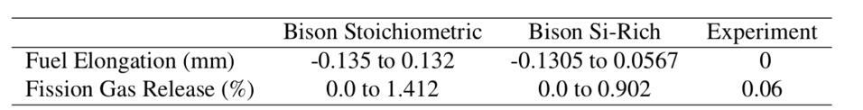
Spearman correlation coefficients
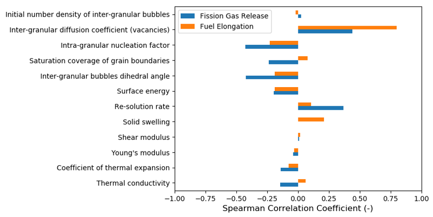
Example of BISON-Dakota Coupling for a Parametric Study
BISON-Dakota coupling can be used for parametric studies (e.g., experiment design)
Here, consider an analysis investigating the affect of a chromium coating on the behavior of Zircaloy cladding tubes.
Problem Description
Parametric study on cladding-only tubes under LOCA-like conditions until failure (an overstrain failure criterion is used).
Used to investigate the reported observation that coated tubes balloon less than uncoated tubes.
0.25 m long, 8.36 mm ID, 0.57 mm thick tubes were used.
Temperature ramped from 300 K to a sinusoid centered about the tube midplane with a 20 K variation, with peak occurring at the tube midplane at 10,000 s.
Pressure ramp beings at 10,000 s.
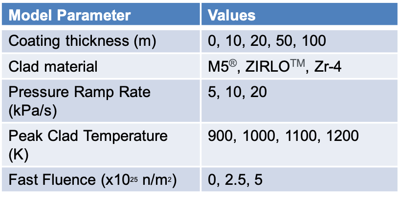
Dakota Input File
# Dakota Input File: Input.in
# Usage:
# dakota –i input.in –o output.out

environment
    tabular_graphics_data

method
  multidim_parameter_study
  partitions = 3 3 2 2

model
    single

variables
  histogram_point_uncertain
    real = 4
    pairs_per_variable = 4 4 3 3
    abscissa = 10.0e-6 20.0e-6 50.0e-6 100.0e-6 900.0 1000.0 1100.0 1200.0 5.0e3 10.0e3 20.0e3 0.0 2.5e25 5.0e25
    counts = 1 1 1 1 1 1 1 1 1 1 1 1 1 1
    descriptors = 'coating_thickness' 'max_temperature' 'pressure_ramp_rate' 'initial_fluence'

interface
  system
    analysis_driver   'run_submission'
    parameters_file   'params.in'
    results_file      'results.out'
      file_save
      file_tag

responses
    response_functions = 1
    descriptors = 'end_time'
    no_gradients
    no_hessians
Results
The time to rupture is longer in the coated cases, indicating smaller balloons at any given time. Results shown for ZIRLO substrate.
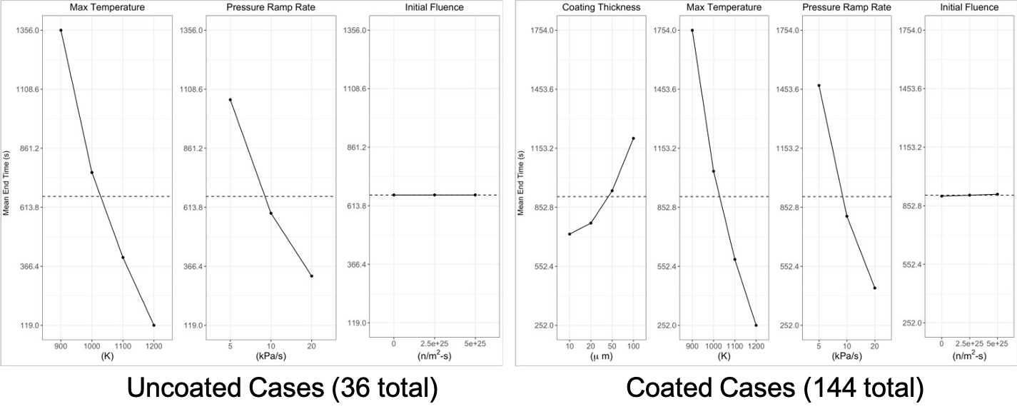
Multiphysics and MultiApp
Why Use a MultiApp System
Multiscale
Microscopic physics affect macroscopic physics which, in turn, affect microscopic physics.
Some physics only exist in part of the domain.
Physics changes at different length scales.
Multi-mesh
Link meshes of different dimensions during a simulation.
Link physics that require a coarser (or finer) mesh than other coupled physics.
Many more that we have not thought of yet.
BISON with MultiApp
MOX Assessment Cases
Formation of central void for tracking porosity
Oxygen diffusion
Metallic Fuel Research
Zirconium diffusion
BISON is just beginning to use this system, so there is more to come.
A MOOSE Framework Tool
Really, the MultiApp system is a MOOSE framework tool that BISON may use.
Let's look at their tutorial (Step 10) to see it in action.
References
- M. M. Rashid. Incremental kinematics for finite element applications. International Journal for Numerical Methods in Engineering, 36:3937–3956, 1993.
- A. M. Ross and R. L. Stoute. Heat transfer coefficient between UO$_2$ and Zircaloy-2. Technical Report AECL-1552, Atomic Energy of Canada Limited, 1962.
- L. Schoof and V. Yarberry. EXODUS II: A finite element data model. Technical Report SAND92-2137, Sandia National Laboratories, September 1996.
- Sandia National Laboratories. CUBIT: geometry and mesh generation toolkit. http://cubit.sandia.gov, 2008.