BISON Developer Workshop
Implicit, parallel, fully-coupled nuclear fuel performance analysis
Computational Mechanics and Materials Department
Idaho National Laboratory
BISON Team Members
Rich Williamson
(Richard.Williamson@inl.gov)Steve Novascone
(Stephen.Novascone@inl.gov)Jason Hales
(Jason.Hales@inl.gov)Ben Spencer
(Benjamin.Spencer@inl.gov)Kyle Gamble
(Kyle.Gamble@inl.gov)Gyanender Singh
(Gyanender.Singh@inl.gov)
Stephanie Pitts
(Stephanie.Pitts@inl.gov)Adam Zabriskie
(Adam.Zabriskie@inl.gov)Aysenur Toptan
(Aysenur.Toptan@inl.gov)Wen Jiang
(Wen.Jiang@inl.gov)Pierre-Clément Simon
(pierreclement.simon@inl.gov)Wenfeng Liu
(Wliu@Structint.com)Christopher Matthews
(cmatthews@lanl.gov)
BISON Overview
Fuel Behavior: Introduction
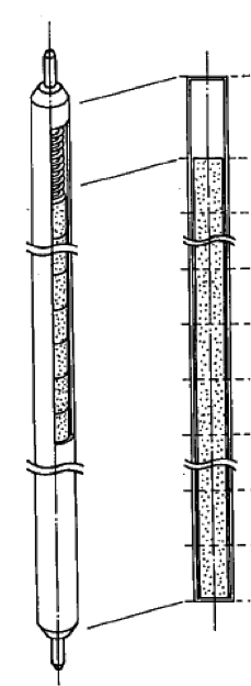
At beginning of life, a fuel element is quite simple...
Nakajima et al., Nuc. Eng. Des., 148, 41 (1994)
but irradiation brings about substantial complexity...
Michel et al., Eng. Frac. Mech., 75, 3581 (2008)
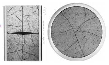
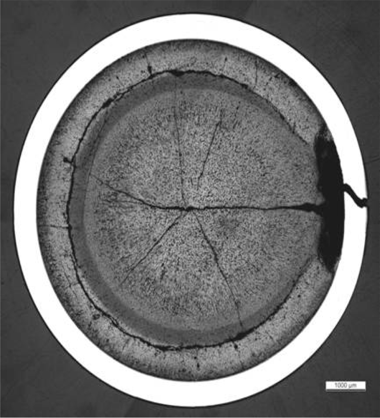
Fuel Fracture
Olander, p. 584 (1978)
Multidimensional Contact
and Deformation
Olander, p. 584 (1978)
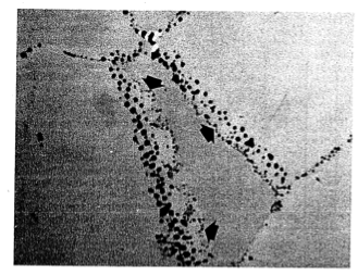
Fission Gas
Bentejac et al., PCI Seminar (2004)
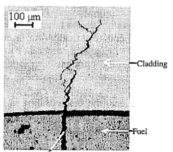
Stress Corrosion
Cracking Cladding
Failure
Fuel Behavior Modeling: Coupled Multiphysics
Multiphysics
Fully coupled nonlinear thermo-mechanics
Multiple species diffusion
Neutronics
Thermal-hydraulics
Chemistry
Multi-space scale
Important physics at the atomistic and micro-structural levels
Practical engineering simulations require the continuum level
Multi-time scale
Steady operation ( week)
Power ramps/accidents
( s)

BISON - Nuclear Fuel Performance Analysis
BISON is a nuclear fuel performance analysis tool. It is used primarily for analysis of fuel but has also been used to model TRISO fuel, both rod and plate metal fuel, and accident tolerant fuel. BISON is built on top of MOOSE.
BISON is implicit
Large time steps
BISON runs in parallel
Runs naturally on one or many processors
BISON is fully coupled
No operator splitting or staggered scheme necessary
All unknowns are solved for simultaneously
BISON is under development; there is still much to do
Fission gas release model continues to improve
Contact can be a challenge; friction needs improvement
Automatic time-stepping needs improvement
Documentation and validation is evolving
BISON's Relationship to MOOSE
Code too specific for MOOSE but useful for multiple applications is collected in libraries.
BISON depends on:
MOOSE modules (solid mechanics, fluid dynamics, etc.) depends on:
MOOSE (multiphysics application framework) depends on:
libMesh (numerical PDE solution framework out of UT Austin) depends on:
PETSc, Exodus II, MPI, etc.
BISON LWR Capabilities
General Capabilities
3D, 2D-RZ, 1D fully coupled thermo-mechanics
Large deformations
Parallel
Meso-scale informed
Oxide Fuel Behavior
Temperature/burnup/porosity dependent material properties
Volumetric heat generation
Thermal and fission product swelling, and densification strains
Thermal and irradiation creep
Fuel fracture via relocation and smeared cracking
Fission gas release (2 stages)
transient release
grain growth/sweeping
athermal release
Temperature
Gap/Plenum Behavior
Gap heat transfer with
Mechanical contact
Plenum pressure as a function of:
evolving gas volume (from mechanics)
gas mixture (FGR)
gas temperature approximation
Cladding Behavior
Thermal and irradiation creep
Thermal expansion
Irradiation growth
Plasticity
Hydride damage
Coolant Channel
Closed channel thermal hydraulics with heat transfer coefficients
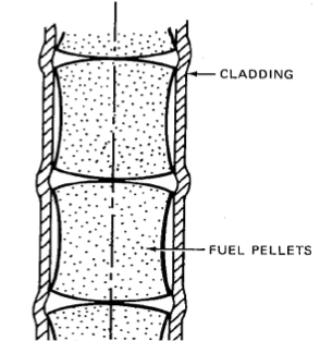
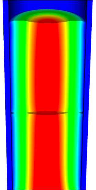
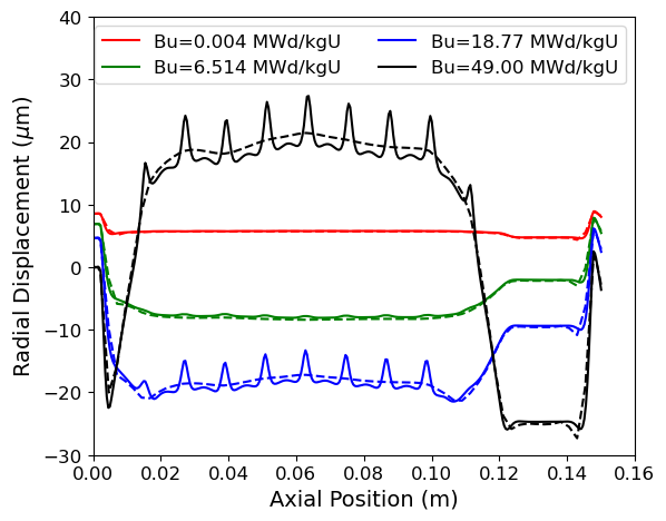
BISON Example - Axisymmetric LWR Fuel Rodlet
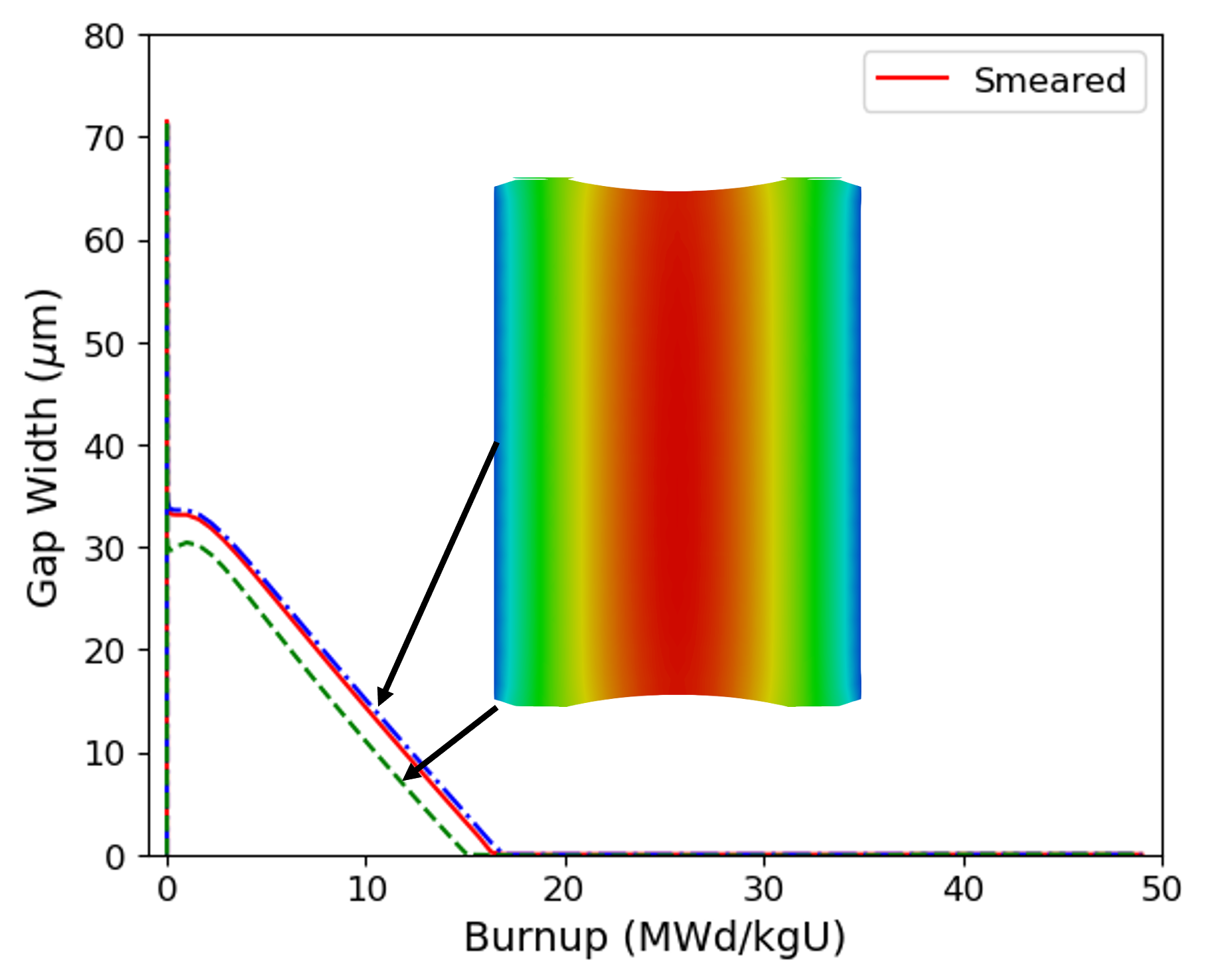
BISON Results - Axisymmetric LWR Fuel Rodlet
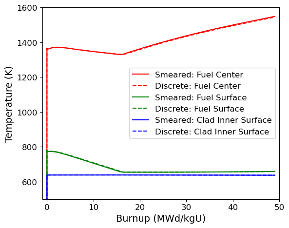
Thermal expansion, fuel densification, clad creep-down, fission gas release, contact, and burnup dependent fuel thermal conductivity all affect fuel temperatures
Hourglass shape of pellets is evident in gap closure histories
BISON Results - Axisymmetric LWR Fuel Rodlet
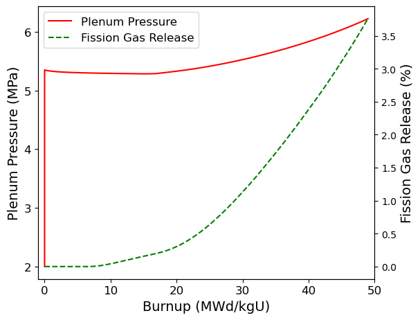
Fission gas release begins at a burnup of 10 MWd/kgU
Hourglass shape of pellets creates ridges in clad during PCMI
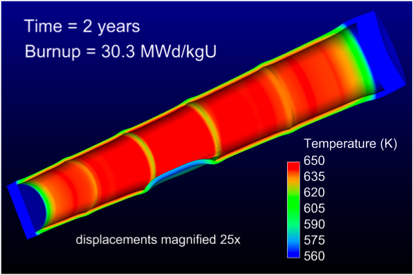
BISON Example - Missing Pellet Surface
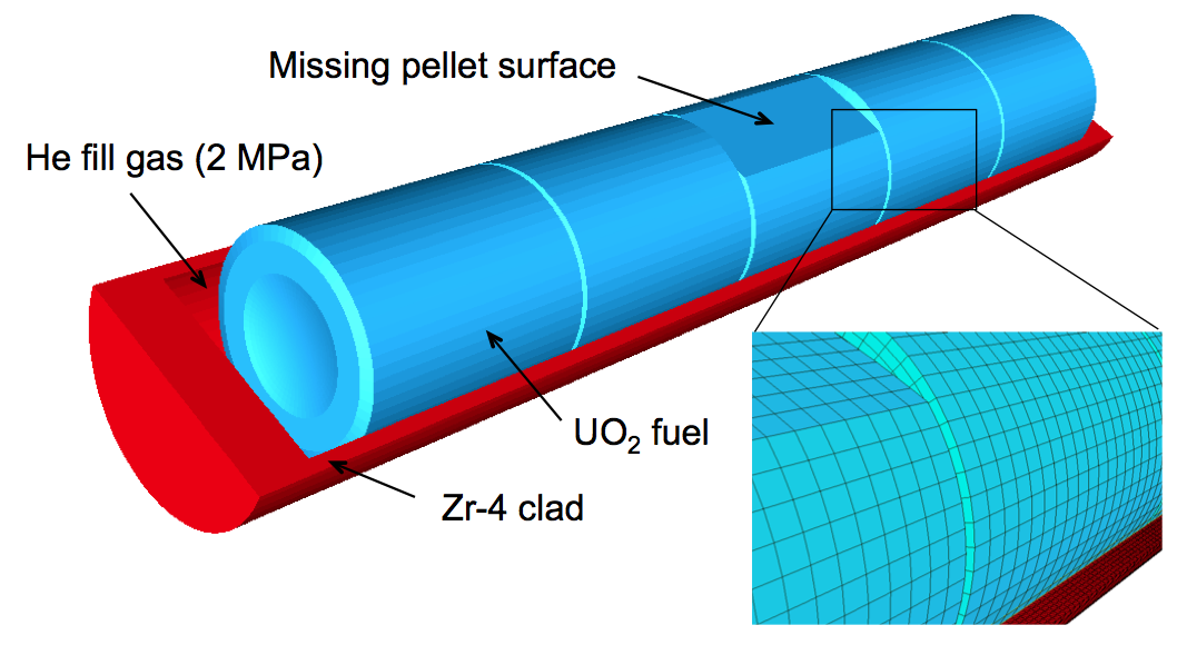
High-resolution 3D calculation (25,000 elements, 1.1 dof) run on 120 processors
Simulation starting from a fresh fuel state with a typical power history, followed by a late-life power ramp
BISON Results - Missing Pellet Surface
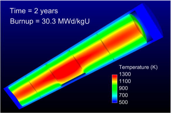
Fuel Temperature
Clad Temperature
Missing pellet surface has a very significant effect on the temperature and stress state in the rod
Model can be used to examine source of rod failures
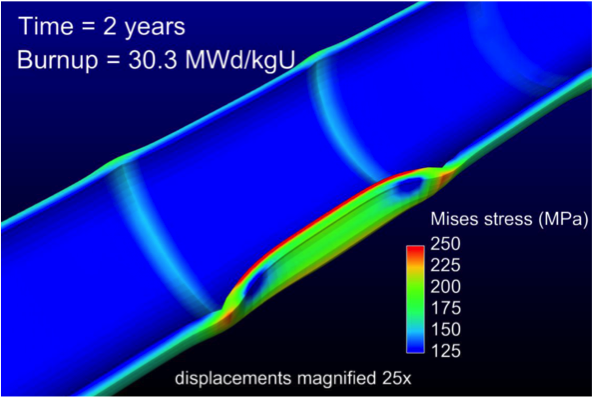
Clad Stress
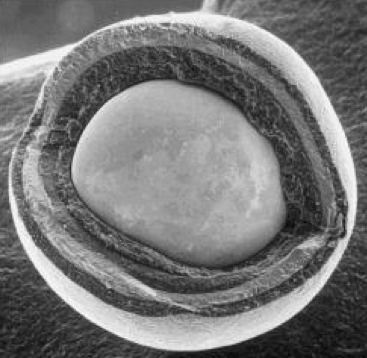
BISON Coated-Particle Fuel Capabilities
General Capabilities
3D, 2D-RZ, 1D fully coupled thermomechanics with species diffusion
Large deformation
Elasticity with thermal expansion
Steady and transient
Massively parallel
Fuel Kernel
Temperature, burnup, porosity dependent conductivity
Solid and gaseous fission product swelling
Densification
Thermal/irradiation creep
Fission gas release
CO production
Radioactive decay
Tangential Stress
Gap Behavior
Gap heat transfer with
Gap mass transfer
Mechanical contact
Plenum pressure as a function of:
evolving gas volume (from mechanics)
gas mixture (FGR and CO)
gas temperature approximation
Silicon Carbide
Irradiation creep
Pyrolytic Carbon
Anisotropic irradiation-induced strain
Irradiation creep
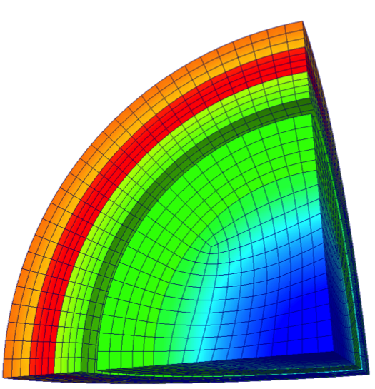
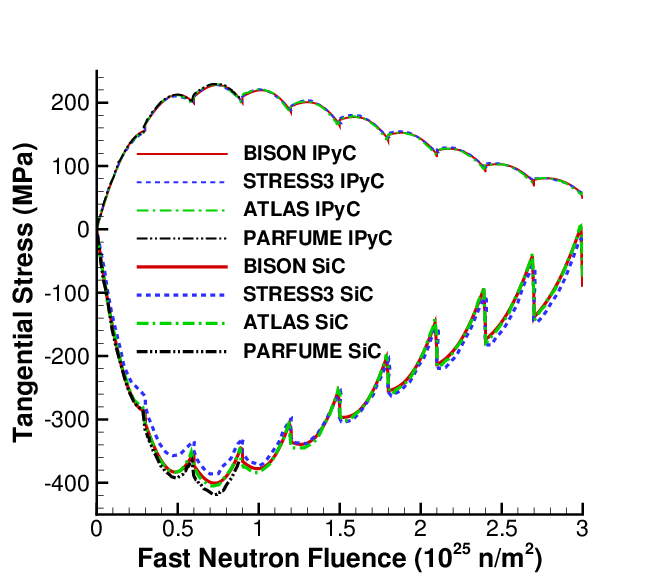
BISON Results - TRISO Particle
Validated against PARFUME, ATLAS, STRESS3
Code comparisons are excellent
Run times of 1 s are typical
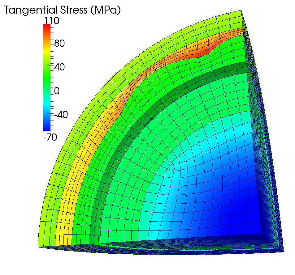
PBR cyclic particle temperature
Aspherical particles are common
Raises peak tensile stress by 4x
Runs in a few minutes (8 procs)
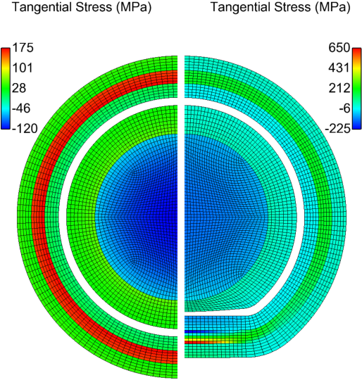
BISON Results - 3D Simulation of Thinned SiC Layer
Localized SiC thinning due to soot inclusions or fission product interaction
3D capability demonstrated on eighth particle with random thinning
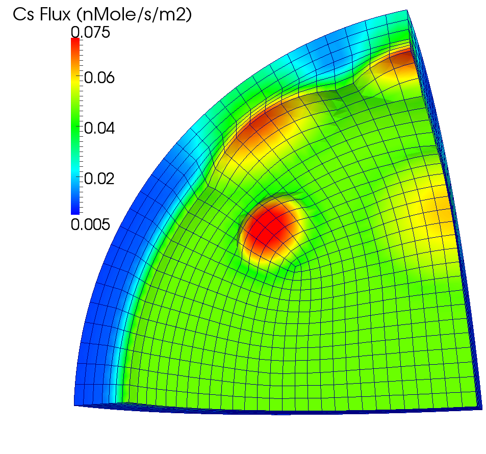
Significantly higher tensile stress and cesium release; impossible to predict with state-of-the-art 1D or 2D analyses
Typical run times of a few hours on 8 procs
Fuels Specific Models
Fuels Specific Models
Bison consists, in addition to the capability in MOOSE, of material models specific to nuclear fuels:
Fission gas release
Material models that are functions of irradiation
Creep
Thermal Conductivity
Relocation
Other models that capture fuel behavior, like radial and axial power profiles
Gap heat transfer in LWR fuel
This section highlights some of these models.
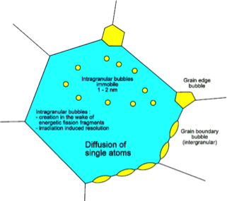
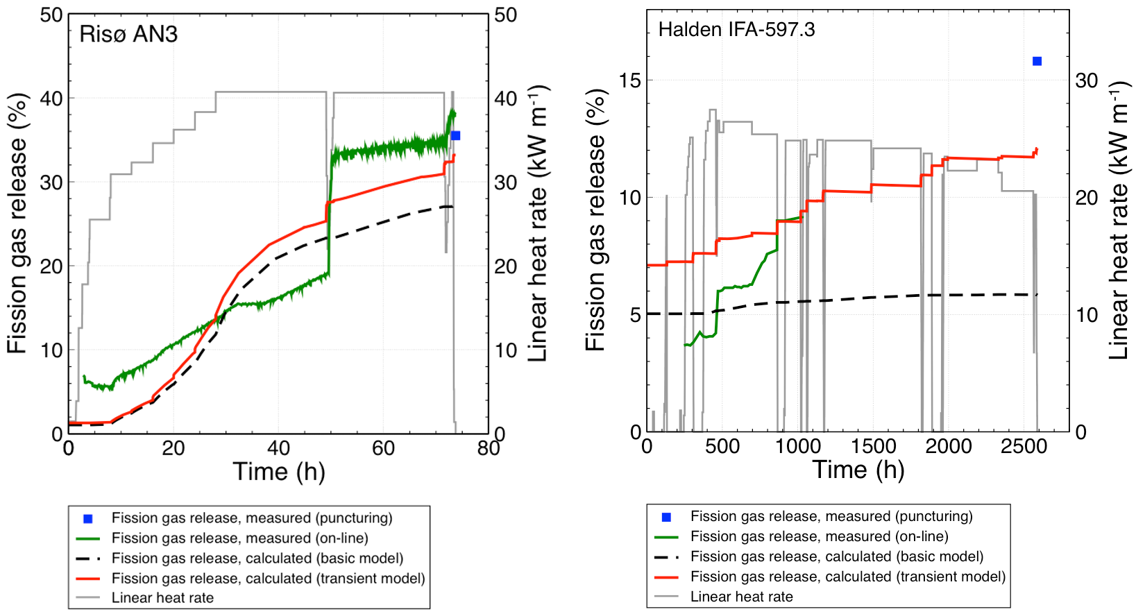
Fission Gas Behavior
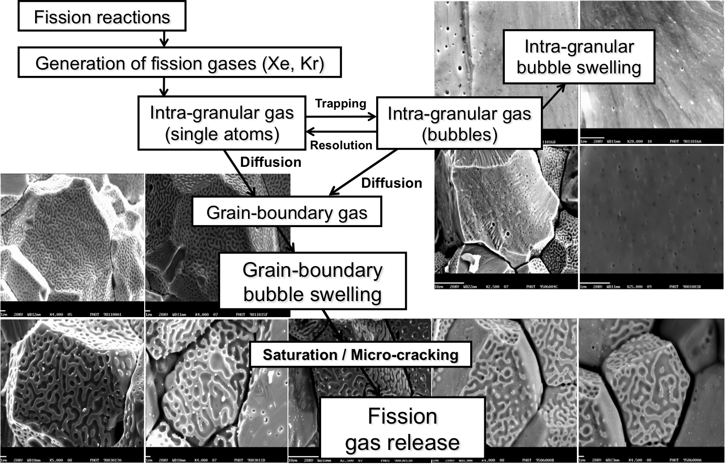
Bison Fission Gas Model
Physics-based model that describes the different stages of fission gas behavior
Gas generation
Intra-granular diffusion to grain boundaries
Bubble development at grain boundaries and associated fuel swelling
Fission gas release due to grain boundary saturation
Fission gas release due to micro-cracking
Current results are state-of-the-art or better
Material Models that Depend on Irradiation or Power
Zirconium, mechanics example:
where
is the effective irradiation creep rate (1/s),
is the fast neutron flux (n/m2-s),
is the effective (Mises) stress (MPa),
and , , and are material constants.
UO, thermal conductivity example:
where the terms of the conductivity are functions of burnup and temperature.
Relocation:
This relocation model is a function of power(), as-fabricated pellet diameter(), as-fabricated gap thickness (), and burnup.
Power Profiles
Radial power profile example:
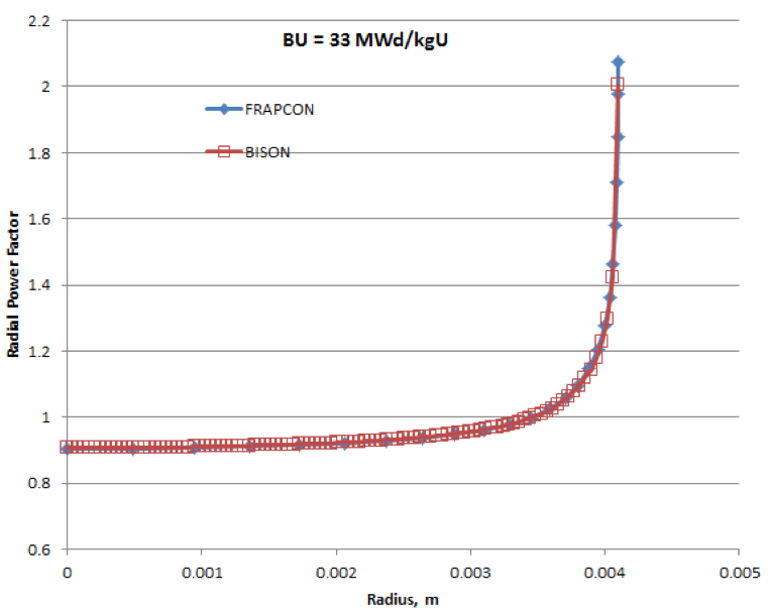
Don't forget the axial profile.
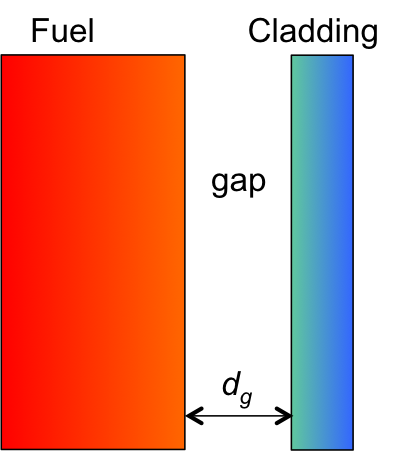
LWR Gap Heat Transfer
In BISON, and are described using the form proposed by Ross and Stoute (1962). is defined as
where is the conductivity of the gas in the gap, is the gap width, is a roughness coefficient, and are roughnesses of the surfaces, and and are jump distances, which become important for small gap widths and low gas pressures. The jump distances provide a reduction in gap conductance when the mean free path of the gas molecules is significant in comparison to the gap width, and the continuum approximation is no longer valid. The gas temperature () is the average of the two surfaces.
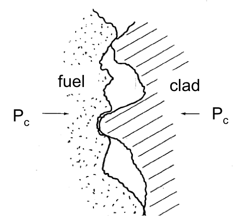
LWR Gap Heat Transfer
is defined as
where is an empirical constant, and are the thermal conductivities of the two materials, is the contact pressure, is the average gas film thickness, and is the Meyer hardness of the softer material.
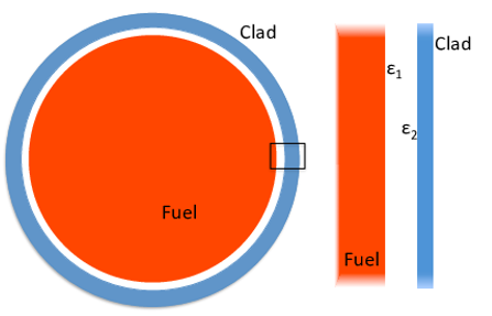
Bison Gap Heat Transfer (continued)
In BISON, is computed using a diffusion approximation. Based on the Stefan-Boltzmann law,
where is the Stefan-Boltzmann constant, is an emissivity function, and and are the temperatures of the radiating surfaces.
The radiant conductance is approximated as
which can be reduced to
For infinite parallel plates,
where and are the emissivities of the radiating surfaces. This is the specific function implemented in BISON.
MOOSE, a Partial Differential Equation Solver
We are interested in solving a set of partial differential equations (PDEs) that represent physical processes, such as heat transfer and solid mechanics.
MOOSE is a general solver that uses the finite element method (FEM) to solve arbitrary sets of PDEs for specific applications.
FEM converts complex PDEs into a set of coupled algebraic equations which can be readily solved on a computer.
FEM is applicable to a wide range of PDEs and can represent problems with arbitrary geometry.
FEM Vocabulary
The following list contains terms commonly used when discussing the finite element approach. These definitions are NOT COMPREHENSIVE. This list is just to get the conversation started.
Domain - The space or geometry of your problem.
Element - To obtain the approximate solution, the domain must be subdivided (discretized) into simpler smaller regions. These are called elements.
Node - The points at which the elements are connected. We typically compute the value of primary solution variables (temperature, displacement) at nodes. Also where Dirichlet boundary conditions are applied.
Boundary Condition - A constraint, or 'load' applied to the domain.
Quadrature Point - One of the steps to finding the approximate solution to the PDE is integration. Quadrature points are where this integration happens. They are located within the elements.
Test or Shape Function - Functions that help form the approximate solution to the PDE.
Heat Conduction
MOOSE Modules' heat conduction routines are built to help solve
where is the mass density, is the specific heat, is the temperature, is the thermal conductivity, and is the volumetric heat generation rate.
MOOSE Modules provides spherically symmetric 1D, axisymmetric 2D, and 3D formulations. Either first or second order elements may be used (QUAD4 or QUAD8 for RZ, HEX8 or HEX20 for 3D).
Heat Conduction Continued
Multiply by test function, integrate
Integrate by parts
Jacobian
The Input File
To solve these PDEs, we need to create an input file that contains all the necessary information.
By default MOOSE uses a hierarchical, block-structured input file.
Within each block, any number of name/value pairs can be listed.
The syntax is completely customizable, or replaceable.
To specify a simple problem, you will need to populate five or six top-level blocks.
We will briefly cover a few of these blocks in this section and will illustrate the usage of the remaining blocks throughout this manual.
The Required Blocks of an Input File
Mesh- the domain of the problemVariables- temperature and displacementKernels- heat conduction, solid mechanicsMaterials- used by kernels, e.g. thermal conductivityBCs- specify Dirichlet or NeumannExecutioner- steady state or transientOutputs- set options for how you want the output to look.
Example Input File
The following input file is an example of how to solve the heat conduction equation with a source term.
[Mesh]
  type = GeneratedMesh
  dim = 2
  nx = 10
  ny = 10
[]

[Variables]
  [./temp]
  [../]
[]

[Kernels]
  [./heat_conduction]
    type = HeatConduction
    variable = temp
  [../]
  [./heat_source]
    type = HeatSource
    variable = temp
    value = 10000
  [../]
[]

[Materials]
  [./heat_conductor]
    type = HeatConductionMaterial
    thermal_conductivity = 1
    block = 0
  [../]
[]
[BCs]
  [./leftright]
    type = DirichletBC
    variable = temp
    boundary = 'left right'
    value = 200
  [../]
[]

[Executioner]
  type = Transient
  solve_type = 'PJFNK'
  petsc_options_iname = '-pc_type -pc_factor_mat_solver_package'
  petsc_options_value = 'lu superlu_dist'
  dt = 1.0
  end_time = 1.0
[]

[Outputs]
  exodus = true
  [./console]
    type = Console
    perf_log = true
  [../]
[]

[Postprocessors]
  [./peak_temp]
    type = NodalExtremeValue
    variable = temp
  [../]
[]
Mesh Block
[Mesh]
  type = GeneratedMesh
  dim = 2
  nx = 10
  ny = 10
[]

The FEM mesh is defined in the block.
A mesh can be read in from a file. There are many accepted formats (see the MOOSE manual). We typically use the exodus file format and create meshes with CUBIT.
Simple meshes can also be generated within the input file. We'll use this approach for our first examples.
The sides of a
GeneratedMeshare named in a logical way (bottom, top, left, right, front, and back).
Variables Block
[Variables]
  [./temp]
  [../]
[]
The primary or dependent variables in the PDEs (temperature, displacement) are defined in the
Variablesblock.A user-selected unique name is assigned for each variable.
Kernels Block
[Kernels]
  [./heat_conduction]
    type = HeatConduction
    variable = temp
  [../]
  [./heat_source]
    type = HeatSource
    variable = temp
    value = 10000
  [../]
[]
The kernels (individual terms in the PDEs being solved) are listed in the
Kernelsblock.Each kernel is assigned a specific variable (in this case, temp or temperature).
Materials Block
[Materials]
  [./heat_conductor]
    type = HeatConductionMaterial
    thermal_conductivity = 1
    block = 0
  [../]
Material properties are defined in the
Materialsblock. Information from the materials block is used by some kernels.Here, thermal conductivity is defined to be used by the
HeatConductionkernel.
Boundary Conditions (BCs) Block
[BCs]
  [./leftright]
    type = DirichletBC
    variable = temp
    boundary = 'left right'
    value = 200
  [../]
[]
Define temperature on boundary
Boundary conditions are defined in the
BCsblock.Many types of boundary conditions can be applied.
For this simple example, the temperature is set on the left and right sides of the domain.
Executioner Block
[Executioner]
  type = Transient

  solve_type = 'PJFNK'
  petsc_options_iname = '-pc_type -pc_factor_mat_solver_package'
  petsc_options_value = 'lu superlu_dist'
  dt = 1.0
  end_time = 1.0
[]
The
Executionerblock defines how the problem is solved.The parameters
solve_typeandpetsc_optionswill be discussed later.
Outputs Block
[Outputs]
  exodus = true
  [./console]
    type = Console
    perf_log = true
  [../]
[]
The results you will output from your simulation are defined in the
Outputsblock.This includes defining the file type (exodus file here).
Performance logs are also defined.
Postprocessors Block
[Postprocessors]
  [./peak_temp]
    type = NodalExtremeValue
    variable = temp
  [../]
[]
Analysis results in the form of single scalar values are defined in the
Postprocessorsblock.May operate on elements, nodes, or sides of the model.
Examples include
NodalExtremeValue,AverageElementSize, andSideAverageValue.
Run Problem and Look at Results with Paraview
The problems shown here can be run either with an application such as Bison that links in the heat_conduction module, or with the MOOSE combined module executable.
To run with the MOOSE combined modules executable, run:
~/projects/moose/modules/combined/combined-opt -i heat_cond.i
To run with an application (Bison example shown here), run:
~/projects/bison/bison-opt -i heat_cond.i
These examples assume your code is in the
~/projectsdirectory. Substitute in an appropriate path if it is located elsewhere.
Heat Conduction with Source: Results

Mechanics
MOOSE modules' mechanics routines are built to help solve:
where is the stress and is a body force.
MOOSE modules also supplies boundary conditions useful for mechanics (such as pressure).
MOOSE modules provides spherically symmetric 1D, axisymmetric 2D (typically linear), and 3D fully nonlinear formulations. Either first or second order elements may be used (QUAD4 or QUAD8 for RZ; HEX8 or HEX20 for 3D).
Mechanics (cont.)
Multiply by test function, integrate
Integrate by parts
Mechanics: Spherically Symmetric 1D
The 1D, 2D, and 3D classes have much in common.
The calculation of the strain is of course different for the three formulations. However, they share material models.
The spherically symmetric 1D strain is
The mesh for spherically symmetric 1D is defined such that the x coordinate corresponds to the radial direction.
No displacement in the x (radial) direction must be explicitly enforced in the input file for nodes at x=0.
Mechanics: Axisymmetric 2D
The axisymmetric 2D strain is
The mesh for RZ is defined such that the x coordinate corresponds to the radial direction and the y coordinate with the axial direction.
No displacement in the x (radial) direction must be explicitly enforced in the input file for nodes at x=0.
Mechanics: Nonlinear 3D
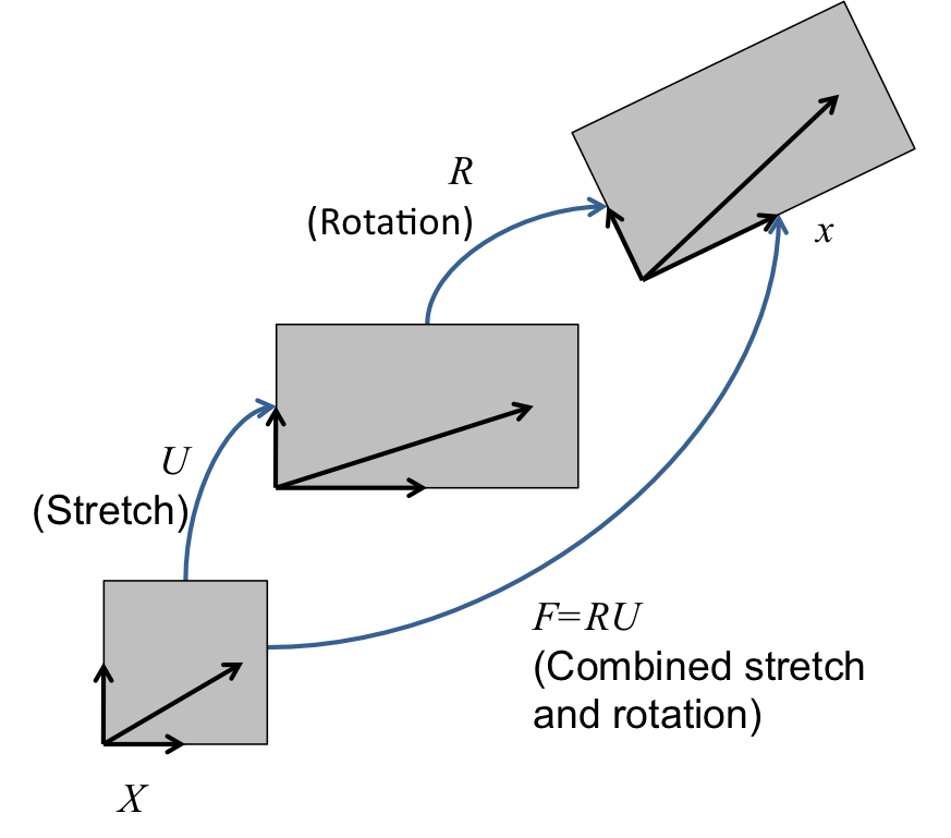
The nonlinear kinematics formulation in MOOSE modules accommodates both large strains and large rotations.
The deformation gradient can be viewed as the derivative of the current coordinates with respect to the original coordinates.
can be decomposed into pure rotation and pure stretch .
Mechanics: 3D
We begin with a complete set of data for step and seek the displacements and stresses at step . We first compute an incremental deformation gradient;
With , we next compute a strain increment that represents the rotation-free deformation from the configuration at to the configuration at . Following Rashid (1993), we seek the stretching rate :
Here, is the incremental stretch tensor, and is the incremental Green deformation tensor. Through a Taylor series expansion, this can be determined in a straightforward, efficient manner.
Mechanics: 3D (cont.)
is passed to the constitutive model as an input for computing at .
The next step is computing the incremental rotation, , where . Like for , an efficient algorithm exists for computing . It is also possible to compute these quantities using an eigenvalue/eigenvector routine.
With and , we rotate the stress to the current configuration.
Mechanics: Material Models
The material models for 1D, axisymmetric 2D, and 3D are formulated in an incremental fashion (think hypo-elastic).
Thus, the stress at the new step is the old stress plus a stress increment:
The incremental formulation is particularly useful for plasticity and creep models.
Let's add some more physics... Mechanics!
The following blocks have to be added to or modified in our input file if we want to include mechanics behavior.
[Variables]
  [./temp]
  [../]
  [./disp_x]
  [../]
  [./disp_y]
  [../]
[]

[Kernels]
  [./TensorMechanics]
    use_displaced_mesh = true
  [../]
  [./heat_conduction]
    type = HeatConduction
    variable = temp
  [../]
  [./heat_source]
    type = HeatSource
    variable = temp
    value = 10000
    function = source
  [../]
[]
Let's add some more physics... Mechanics!
The following blocks have to be added to or modified in our input file if we want to include mechanics behavior.
[Materials]
  [./heat_conductor]
    type = HeatConductionMaterial
    thermal_conductivity = 1
    block = 0
  [../]
  [./elasticity_tensor]
    type = ComputeIsotropicElasticityTensor
    block = 0
    youngs_modulus = 1e6
    poissons_ratio = 0.3
  [../]
  [./thermal_expansion_strain]
    type = ComputeThermalExpansionEigenstrain
    stress_free_temperature = 200
    thermal_expansion_coeff = 1.0e-4
    temperature = temp
    eigenstrain_name = thermal_eigenstrain
    block = 0
  [../]
  [./strain]
    type = ComputeFiniteStrain
    block = 0
    eigenstrain_names = thermal_eigenstrain
  [../]
  [./stress]
    type = ComputeFiniteStrainElasticStress
    block = 0
  [../]
[]
Let's add some more physics... Mechanics!
The following blocks have to be added to modified in our input file if we want to include mechanics behavior.
[BCs]
  [./leftright_temp]
    type = DirichletBC
    variable = temp
    boundary = 'left right'
    value = 200
  [../]
  [./leftright_disp_x]
    type = DirichletBC
    variable = disp_x
    boundary = 'left right'
    value = 0
  [../]
  [./bottom_disp_y]
    type = DirichletBC
    variable = disp_y
    boundary = bottom
    value = 0
  [../]
[]
Heat Conduction + Mechanics: Results

Modules: Contact: Finite Element Contact Basics
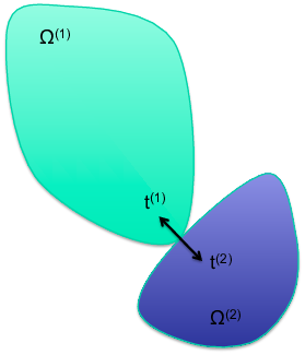
A contact capability in a solid mechanics finite element code prevents the penetration of one domain into another, or part of one domain into itself.
Modules: Contact: Required Capabilites
A necessary but insufficient list:
Search
Exterior identification
Nearby nodes
Capture box
Binary search, e.g.
Contact existence
More geometric work
Penetration point
Enforcement
Formulation of contact force
Formulation of Jacobian
Interaction with other capabilities
Contact: Overview
In node-face contact, nodes (green) may not penetrate faces (defined by orange nodes).
Forces must be determined to push against the two contacting bodies.
No force should be applied where the bodies are not in contact.
The contact forces must increase from zero as the bodies first come into contact.

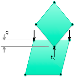
Contact: Constraints
; the gap (penetration distance) must be non-positive
; the contact force must push bodies apart
; the contact force must be zero if the bodies are not in contact
; the contact force must be zero when constraints are formed and released
The gap in the normal direction for constraint is ( is the normal, denotes normal direction, is position of the slave node, is position of the contact point, and is a matrix):
Contact: Contact Options
formulation: kinematicorpenaltyKinematic is more accurate but also harder to solve.
model:frictionless, glued, orcoulombFrictionless enforces the normal constraint and allows nodes to come out of contact if they are in tension. Glued ties nodes where they come into contact with no release. Coulomb is frictional contact with release.
friction_coefficientCoulomb friction coefficient.
penaltyThe penalty stiffness to be used in the constraint.
primaryThe surface corresponding to the faces in the constraint.
secondaryThe surface corresponding to the nodes in the constraint.
normal_smoothing_distanceDistance from face edge in parametric coordinates over which to smooth the normal. Helps with convergence. Try 0.1.
tension_releaseThe tension value that will allow nodes to be released. Defaults to zero.
Even more physics... CONTACT
The following blocks have to be added to or modified in our input file if we want to include the effects of mechanical contact.
[Mesh]
  file = contact.e
  displacements = 'disp_x disp_y'
[]

[Functions]
  [./source]
  type = PiecewiseLinear
  x = '0 1'
  y = '0 1'
  [../]
[]

[Kernels]
.
.
  [./heat_source]
    type = HeatSource
    variable = temp
    value = 1500
    function = source
    block = 2
  [../]
.
.
[Contact]
  [./mechanical]
    master = 1
    slave = 7
    disp_x = disp_x
    disp_y = disp_y
    penalty = 1e7
    tangential_tolerance = 0.1
  [../]
[]
[BCs]
.
.
  [./bottom_disp_y]
    type = DirichletBC
    variable = disp_y
    boundary = 3
    value = 0
  [../]
  [./bottom_disp_y_upper]
    type = DirichletBC
    variable = disp_y
    boundary = '5 6 8'
    value = 0
  [../]
.
.
[]
[Preconditioning]
  [./smp]
    type = SMP
    full = true
  [../]
[]
[Executioner]
  type = Transient
  solve_type = 'PJFNK'
  petsc_options = '-snes_ksp_ew'
  petsc_options_iname = '-pc_type -pc_factor_mat_solver_package'
  petsc_options_value = 'lu superlu_dist'
  line_search = none
  dt = 0.1
  dtmin = 0.01
  num_steps = 10
  nl_rel_tol = 1e-8
  nl_abs_tol = 1e-8
[]
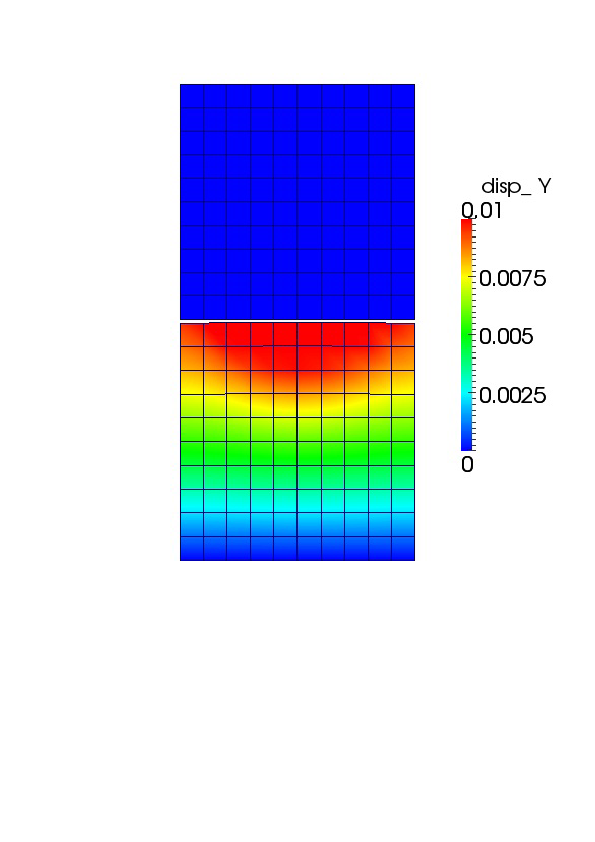
Heat Conduction + Mechanics + Contact: Results
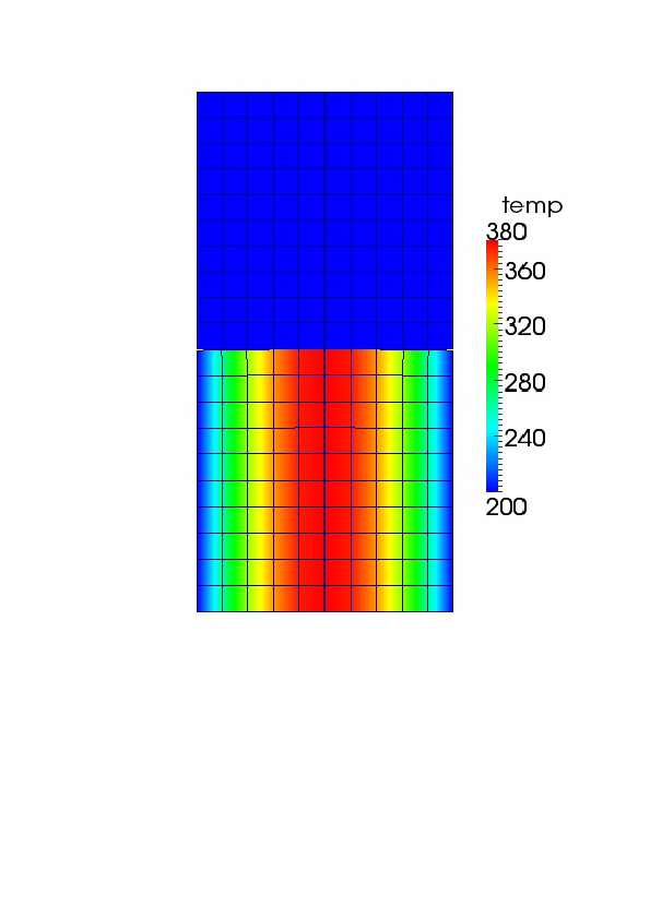
q = 600
Bottom block heats and expands upward, but is not yet in contact
Blocks do not communicate thermally (no gap heat transfer)

Heat Conduction + Mechanics + Contact: Results
q = 600
Bottom block heats and expands upward, but is not yet in contact
Vertical displacement plots show curvature of top surface
Heat Conduction + Mechanics + Contact: Results
q = 1500
Further heating and upward expansion brings blocks into contact; first at the center where the bottom block is hottest
Still, blocks do not communicate thermally (no gap heat transfer)
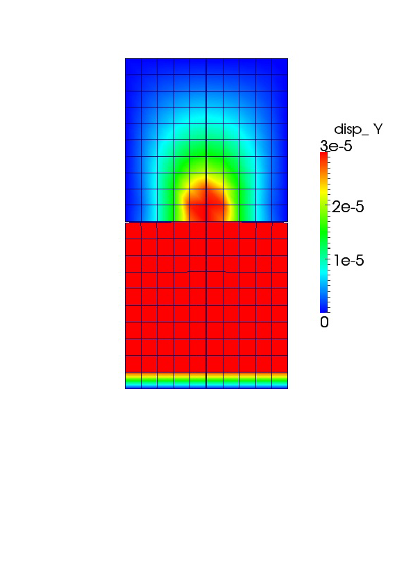
Heat Conduction + Mechanics + Contact: Results
q = 1500
Contour scale is set to show displacement in top block resulting from mechanical contact
Modules: Heat Conduction: Gap Heat Transfer
The principle is that the heat leaving one body must equal that entering another. For bodies and with heat transfer surface :
Gap heat transfer is modeled using the relation:
where is the total conductance across the gap, is the gas conductance, is the increased conductance due to solid-solid contact, and is the conductance due to radiant heat transfer.
In MOOSE modules, only the gas conductance is active by default.
The form of in MOOSE modules is:
where is the conductivity in the gap and is the gap distance.
Adding Thermal Contact
[ThermalContact]
  [./thermal_contact]
    type = GapHeatTransfer
    variable = temp
    master = 1
    slave = 7
    gap_conductivity = 1
  [../]
[]
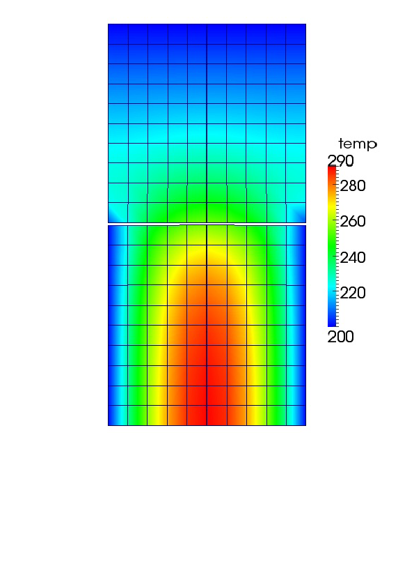
Heat Conduction + Mechanics + Contact + Thermal Contact: Results
q = 750
Heat tranfer occurs through the gap medium prior to mechanical contact
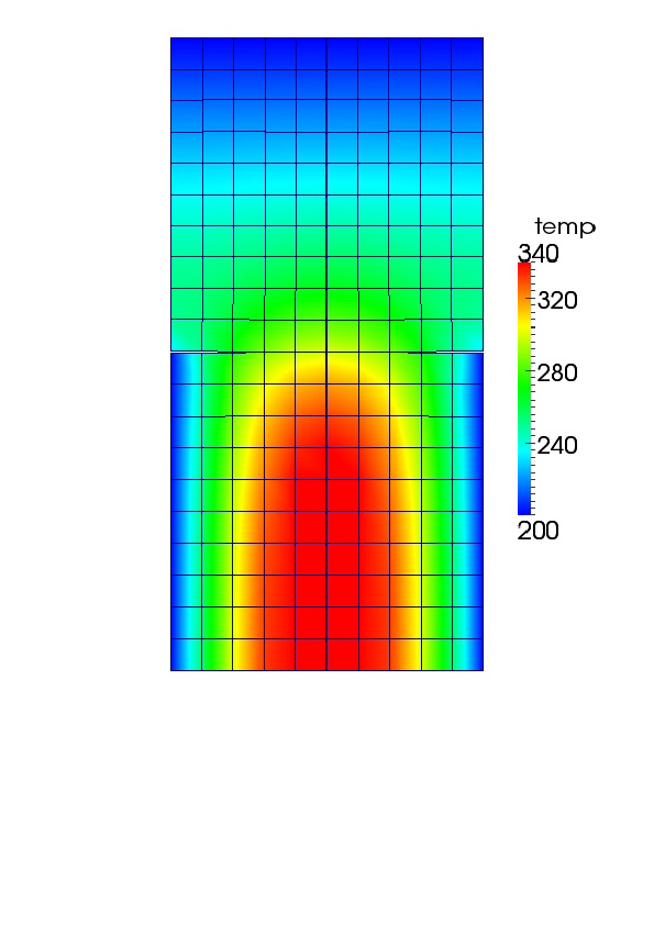
Heat Conduction + Mechanics + Contact + Thermal Contact: Results
q = 1330
Combined thermal and mechanical contact
Running Bison
Running Bison
This section walks through the steps of running Bison on a new problem.
We will build upon the sections describing the input file and mesh generation.
Running Bison ... continued
Let's assume that we want to run a problem similar to the example problem but with the following differences:
Smeared fuel pellet mesh
Coolant pressure of 16 MPa
Rod averaged linear power of 21 kW/m
Clad properties:
- Thermal conductivity of 21.5 W/m/K
- Specific heat capacity of 285 J/kg/K
- Density of 6560 kg/m
- Young's modulus of 99.3 GPa
- Poisson's ratio of 0.37
First, copy the example problem to a new file:
-
mkdir bison/sandbox-cd bison/sandbox-cp ../tensor_mechanics/examples/2D-RZ_rodlet_10pellets/inputQuad8.i myProblem.iNow, in a text editor, we can change the input file.
Editing the Input File: Mesh
Before: inputQuad8.i
# Import mesh file
[Mesh]
  file = quad8Medium10_rz.e
  displacements = 'disp_x disp_y'
  patch_size = 1000 # For contact algorithm
[]
After: myProblem.i
# Import mesh file
[Mesh]
  file = $\alert{coarse1\_rz.e}$
  displacements = 'disp_x disp_y'
  patch_size = 1000
[]
Editing the Input File: Functions
Before: inputQuad8.i
# Define functions to control power, etc.
[Functions]

  [./power_history]
    type = PiecewiseLinear
    data_file = powerhistory.csv
    scale_factor = 1
  [../]

  [./axial_peaking_factors]
    type = PiecewiseBilinear
    data_file = peakingfactors.csv
    scale_factor = 1
    axis = 1 # (0,1,2) => (x,y,z)
  [../]

  [./pressure_ramp]
    type = PiecewiseLinear
    x = '-200 0'
    y = '   0 1'
  [../]

  [./q]
    type = CompositeFunction
    functions = 'power_history
                 axial_peaking_factors'
  [../]
[]
After: myProblem.i
# Define functions to control power, etc.
[Functions]

  [./power_history]
    type = PiecewiseLinear
    $\alert{x = '0 1e4'}$
    $\alert{y = '0 21000'}$
  [../]

  [./axial_peaking_factors]
    type = PiecewiseBilinear
    data_file = peakingfactors.csv
    scale_factor = 1
    axis = 1 # (0,1,2) => (x,y,z)
  [../]

  [./pressure_ramp]
    type = PiecewiseLinear
    x = '-200 0'
    y = '   0 1'
  [../]

  [./q]
    type = CompositeFunction
    functions = 'power_history
                 axial_peaking_factors'
  [../]
[]
Editing the Input File: Coolant Pressure
Before: inputQuad8.i
[./Pressure]
#  apply coolant pressure on clad outer walls
    [./coolantPressure]
      boundary = '1 2 3'
      factor = 15.5e6
      function = pressure_ramp
    [../]
  [../]
After: myProblem.i
[./Pressure]
#  apply coolant pressure on clad outer walls
    [./coolantPressure]
      boundary = '1 2 3'
      factor = $\alert{16e6}$
      function = pressure_ramp
    [../]
  [../]
Editing the Input File: Cladding
Before: inputQuad8.i
[./clad_thermal]
    type = HeatConductionMaterial
    block = clad
    thermal_conductivity = 16.0
    specific_heat = 330.0
  [../]
After: myProblem.i
[./clad_thermal]
    type = HeatConductionMaterial
    block = clad
    thermal_conductivity = $\alert{21.5}$
    specific_heat = $\alert{285.0}$
  [../]
Editing the Input File: Cladding Continued
Before: inputQuad8.i
[./clad_elasticity_tensor]
    type = ZryElasticityTensor
    block = clad
  [../]
After: myProblem.i
[./clad_elasticity_tensor]
    type = $\alert{ComputeIsotropicElasticityTensor}$
    block = clad
    youngs_modulus = $\alert{9.93e10}$
    poissons_ratio = $\alert{0.37}$
  [../]
Editing the Input File: Cladding Continued
Before: inputQuad8.i
[./clad_density]
    type = StrainAdjustedDensity
    block = clad
    strain_free_density = 6551.0
  [../]
After: myProblem.i
[./clad_density]
    type = StrainAdjustedDensity
    block = clad
    strain_free_density = $\alert{6560.0}$
  [../]
Copy Input Data Files
The input file uses a PiecewiseBilinear function (
axial_peaking_factors) that requires a comma separated value (csv) file. PiecewiseBilinear functions allow data lookup in a table.-
cp ../tensor_mechanics/examples/2D-RZ*/peakingfactors.csv .The format of this csv file is as follows:
| coor_1 | coor_2 | coor_3 | ... | coor_M | |
|---|---|---|---|---|---|
| time_1 | factor11 | factor12 | factor13 | ... | factor1M |
| time_2 | factor21 | factor22 | factor23 | ... | factor2M |
| time_N | factorN1 | factorN2 | factorN3 | ... | factorNM |
Generate Smeared Pellet Mesh
With the input file (
myProject.i) complete and the csv file in place, all that remains is to generate the mesh file:-
cp ../tools/UO2/mesh_script.sh .-cp ../tools/UO2/mesh_script.py .-cp ../tools/UO2/mesh_script_input.py coarse1_rz.py-./mesh_script.sh -i coarse1_rz.py
Note, you'll also have to modify the burnup block and axial profile to account for the change in fuel height from 10 pellets to one pellet.
Run Bison
We will now analyze this problem using Bison.
We will use four processors with MPI (Message Passing Interface):
-
mpiexec -n 4 ../bison-opt -i myProblem.iTo run with a single processor:
-
../bison-opt -i myProblem.i
References
- M. M. Rashid. Incremental kinematics for finite element applications. International Journal for Numerical Methods in Engineering, 36:3937–3956, 1993.
- A. M. Ross and R. L. Stoute. Heat transfer coefficient between UO$_2$ and Zircaloy-2. Technical Report AECL-1552, Atomic Energy of Canada Limited, 1962.